Regression with Julia

Today we’ll be taking a quick look at how to do regressions in Julia. But instead of using our advanced knowledge of Flux, or using a pre-made model from GLM.jl. We’ll use the bare basics, and hand-roll a naive toy regression. So as to show you how you yourself can use these basic tools and make your own models rather than being dependent.

For the purpose of this tutorial, instead of picking meaningful data, and carefully working with it, we’ll take random data, and purposefully overfit to it in order to lay bare the workings.

First of all, we’ll import Flux and Gadfly, for ease of differentiation and plotting respectively:

using Flux
using Gadfly

Now we’ll define our simple model to have just one dense layer, but we’ll not use Flux for this purpose, and instead do it ourselves:

model(X) = W*X .+ b

Let’s initialise all our variables to have random values:

function init(n::Int)
	W = rand(n)
	b = zeros(n)
	X, y = rand(n), rand(n)
	return W,b,X,y
end
W,b,X,y=init(100)

We also must define a loss function, so we’ll go with our trusty Euclidean norm:

loss(W,b,X,y) = sum(((W.-X).^2).+((b.-y).^2))

Now we introduce our only usage of Flux in this article:

d = gradient(() -> loss(W,b,X,y), params(W, b))

This stores the derivative of W and b in d. We then extract this derivative compactly via implicit destructuring:

dW,db = d[W],d[b]

Now. we update our weights and biases using a learning rate of 0.01:

W .-= 0.01 * dW
b .-= 0.01 * db

Also, we store the loss in a variable so that Pluto shows it to us easily:

l=loss(W,b,X,y)

Finally, we’ll plot using Gadfly, as the chosen problem lends itself particularly well to visualization:

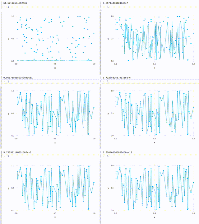
plot(layer(x=X,y=y),layer(x=W,y=b,Geom.line))

And that’s it, you can take my word for this. working, and have the following animation as proof:

Or you can check our the code yourself at the following link:

https://github.com/mathmetal/Misc/blob/master/MLG/SimpleRegression.jl