Linear Programming using Pyomo

Learn how to use Pyomo Packare to solve linear programming problems.

In recent years, with the increase of data and complexity of problems lots of business problems such as food delivery, delivery of online purchase items, and finding an optimum route for cab services, need operations research techniques to optimize their operations. 

In this article, we will focus on the Pyomo Python library. Pyomo is a general-purpose and open-source mathematical modeling package in Python.

Linear Programming

Linear programming is one of the most widely used techniques of operations research for optimizing expenditure, cost, profit, revenue, and resource allocation. Linear programming has wide applicability in production planning, finance, resource allocation, and logistics.

Linear programming finds the optimum value maximum or minimum value for any optimization problem of a linear function with several variables known as decision variables(objective function) subject to satisfying the conditions(constraints). These constraints are non-negative and linear inequalities or constraints.

Historical Context

Linear Programming was invented during World War II to utilize resources in an optimum way. in 1941, Russian mathematician, L. Kantorovich and the American economist, F. L. Hitchcock both developed it independently to solve the transportation problem. Later, G. Stigler developed another linear programming model for solving the balanced diet problem in 1945 and American economist, G. B. Dantzig developed an iterative method to solve linear programming problems known as the simplex method in 1947. 

Terminologies 

• Decision Variables: These variables are defined by you for determining the optimum value. e.g. furniture company wants to determine the optimum number of chair and table units to produce. 
• Objective Function: A linear function that uses decision variables to express goals.
• Constraints: linear math expressions that describe the limitation or restriction on decision variables. Constraints are typically represented as linear inequalities.
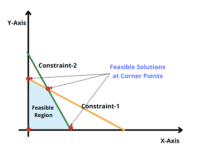
• Feasible Region: A region determined by all the constraints and non-negativity constraints. 
• Feasible solution: feasible solution found on corner points of the feasible region. Corner points are the intersection of boundary liens.
• infeasible solution: Any point outside the feasible region. 
• Optimal Solution: Any point in the feasible region/feasible solutions that gives the optimal value (maximum or minimum) of the objective function. 

Formulate the Problem:

1. Understand the problem 
2. Identify the decision variables (e.g. x, y)
3. Define the objective function expressing the quantity you want to optimize as a linear expression(e.g. z = 3x + 2y). 
4. Define constraints based on the limitations or restrictions of your problem (e.g. x+y = < 60, 2x + y <20).
5. Define Non-Negativity constraints for decision variables e.g. x >= 0 and y>= 0.

Pyomo 

There are various excellent optimization Python packages available such as SciPy, PuLP, Gurobi, Pyomo, ortools, and CPLEX. Pyomo is one of the powerful optimization modeling languages that help us formulate, solve, and analyze mathematical models using Python.

Pyomo stands for Python Optimization Modeling Objects. Pyomo provides the formulation and analysis of complex optimization problems. Modeling comprises the formulation of real-world systems into mathematical equations. Mathematical Modeling is a fundamental process of various scientific research, engineering operations, and business activities.

Pyomo Installation

Let’s first install the Pyomo. You can easily install Pyomo using the pip command. 

pip install pyomo

After installing pyomo, you need to install the GLPK solver. To install it on Windows, you need to download it from the link and set the environment variable for that folder. For detailed window installation please follow this StackOverflow link.

For installing on Linux (e.g. Ubuntu), Open a terminal and install the following link:

sudo apt-get install glpk-utils

You can check your installation by running the following command:

glpsol --help

Solve the Production Planning Problem

An electronics company producing the two products A and B. The company’s new plant can work 105 hours per week. Products A and B take 2 and 3 hours, respectively, for production and packaging. Each product contributes a profit of $40 and $80, respectively. The company’s sales team has determined the maximum sales of 30 and 20 units every week for products A and B, respectively. We need to determine the optimum number of units for products A and B to maximize profits.

Formulate Problem

In this step, we first convert the business problem into the mathematical linear programming format. Let’s assume a and b are two decision variables. Our mathematical formulation is as follows:

Profit Max Z = 40 * a+ 80 *b

Subject to the constraints

Plant Capacity: 2a + 3b ≤ 105 

Sales of Product A: a ≤ 30

Sales of Product B: b≤ 20

Initialize Model

In this step, we will import all the classes and functions of pyomo module and create a model using the ConcreteModel class.

from pyomo.environ import *

# Create a Pyomo model object
model = ConcreteModel()

Define Decision Variable

In this step, we will define the decision variables. In our problem, we have two products A and B. Let’s create them using Var class. Varwill take one argument within.

# Define decision variables
model.a = Var(within=Integers)
model.b = Var(within=Integers)

Define Objective Function

In this step, we will define the maximum objective function by adding it to the Objective class.

# Define objective function for mximum total Profit
model.obj = Objective(expr = 40*model.a + 80*model.b, sense=maximize)

Define the Constraints

In this step, we will add the 3 constraints defined in the problem by adding them to the model object using add() method.

# create ConstraintList object
model.constraints = ConstraintList()

# Define constraints
model.constraints.add(expr = 2*model.a + 3*model.b <= 105) # Plant
model.constraints.add(expr = model.a <= 30) # For Product A
model.constraints.add(expr = model.b <= 20) # For product B

Solve Model

In this step, we will solve the LP problem by calling SolvingFactory class. First, we create the solver using the SolvingFactory class by passing the GLPK solver and then call the solve() method with model oobject as input.

from pyomo.opt import SolverFactory

# Create a solver object
solver = SolverFactory('glpk')

# Solve the LP problem and assign output to results
results = solver.solve(model)

Let’s print the optimum values of the number of units from product A and product B:

# Print the optimal values of the number of units for product A and Product B

print(f"Product A = {model.a.value}")
print(f"Product B = {model.b.value}")
print(f"Profit = {model.obj.expr()}")

Output:
Product A = 24.0
Product B = 19.0
Profit = 2480.0

From the above output, we can say that the optimum number of units for Product A and Product B are 24 and 19 units. The overall maximum profit will be $2480.

Summary

Congratulations, you have made it to the end of this tutorial!

In this article, we have learned Linear Programming, historical context, terminologies, problem formulation, and implementation of Production planning problems in the Python Pyomo library. We have solved the Production Planning problem using Linear Programming with the Pyomo module. Of course, this is just the beginning, and there is a lot more that we can do using Pyomo in Optimization and Supply Chain. In upcoming articles, we will write more on different optimization problems and their solutions using Python. You can check other articles on optimization here.