Solving Linear Programming using Python PuLP

Learn how to use Python PuLP to solve linear programming problems.

As a Senior operation manager, your job is to optimize scarce resources, improve productivity, reduce cost, and maximize profit. For example, you want to maximize the profit of the manufacturing unit with constraints like labor working hours, machine capacity, and available raw material. Another example is that of a marketing manager who wants to allocate the optimum budget among alternative advertising media channels such as radio, television, newspapers, and magazines. Such problems can be considered optimization problems.

Optimization problems can be represented as a mathematical function that captures the tradeoff between the decisions that need to be made. The feasible solutions to such problems depend upon constraints specified in mathematical form.

Linear programming is the core of any optimization problem. It is used to solve a wide variety of planning and supply chain optimization. Linear programming was introduced by George Dantzig in 1947. It uses linear algebra for determining the optimal allocation of scarce resources.

In this tutorial, we are going to cover the following topics:

Linear Programming

LP models are based on linear relationships. It assumes that the objective and the constraint function in all LPs must be linear. This mathematical technique is used to solve the constrained optimization problem.  There are 4 basic assumptions of LP models:

• Additivity Assumption: The terms of objective function and constraints must be additive. e.g. total consumption must equal to sum of the profits from each decision variable and total contributions to the problem objective, resulting in carrying out each activity independently.
• Proportionality Assumption: Each decision variable has a linear impact on the linear objective function and in each constraint.  The consumptions and contributions for each activity are proportional to the actual activity level.
• Divisibility Assumption: Decision variables may accept the non-integer value. Each variable is allowed to have fractional values (continuous variables).
• Certainty Assumption: Each coefficient of the objective vector and constraint matrix is known with certainty (not a random variable) (https://link.springer.com/book/10.1007/978-3-319-68837-4). Model parameters are known and constrained. Relevant constraints have been identified and represented in the model.

Methods for Solving Linear Programming Problems

These are the following methods used to solve the Linear Programming Problem:

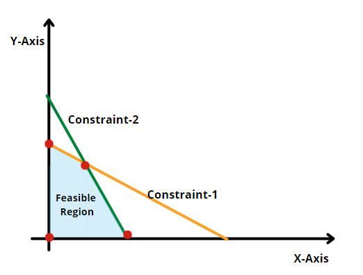
• Graphical Method
• Simplex Method
• Karmakar’s Method

Graphical is limited to the two-variable problem while Simplex and Karmakar’s method can be used for more than two variables.

Components of Linear Programming

• Decision Variables: What you can control.
• Objective Function: math expressions that use variables to express goals.
• Constraints: math expressions that describe the limit of a solution.

Modeling Linear Programming Using Python PuLP

There are various excellent optimization Python packages are available such as SciPy, PuLP, Gurobi, and CPLEX. In this article, we will focus on the PuLP Python library. PuLP is a general-purpose and open-source Linear Programming modeling package in Python.

Install pulp package:

 !pip install pulp

PuLP modeling process has the following steps for solving LP problems:

• Initialize Model
• Define Decision Variable
• Define Objective Function
• Define the Constraints
• Solve Model 

Understand the problem

This problem is taken from Introduction to Management Science By Stevenson and Ozgur.

A furniture company produces a variety of products. One department specializes in wood tables, chairs, and bookcases. These are made using three resources labor, wood, and machine time. The department has 60 hours of labor available each day, 16 hours of machine time, and 400 board feet of wood. A consultant has developed a linear programming model for the department.

x1= quantity of tables

x2= quantity of chairs

x3= quantity of bookcases

Objective Function: Profit = 40*x1+30*x2+45*x3

Constraints:

• labor: 2*x1 + 1*x2 + 2.5*x3 <= 60 Hours
• Machine: 0.8*x1 + 0.6*x2 + 1.0*x3 <= 16 Hours
• Wood: 30*x1 + 20*x2 + 30*x3 <= 400 board-feet
• Tables: x1>=10 board-feet
• x1, x2, x3 >= 0

Initialize Model

In this step, we will import all the classes and functions of pulp module and create a Maxzimization LP problem using LpProblem class.

# Import all classes of PuLP module
from pulp import *

# Create the problem variable to contain the problem data
model = LpProblem("FurnitureProblem", LpMaximize)

Define Decision Variable

In this step, we will define the decision variables. In our problem, we have three variables wood tables, chairs, and bookcases. Let’s create them using LpVariable class. LpVariable will take the following four values:

• First, the arbitrary name of what this variable represents.
• Second is the lower bound on this variable.
• Third is the upper bound.
• Fourth is essentially the type of data (discrete or continuous). The options for the fourth parameter are LpContinuous or LpInteger.

# Create 3 variables tables, chairs, and bookcases

x1 = LpVariable("tables", 0, None, LpInteger)
x2 = LpVariable("chairs", 0, None, LpInteger) 
x3 = LpVariable("bookcases", 0, None, LpInteger)

Define Objective Function

In this step, we will define the maximum objective function by adding it to the LpProblem object.

# Create maximize objective function
model += 40 * x1 + 30 * x2 + 45 * x3 

Define the Constraints

In this step, we will add the 4 constraints defined in the problem by adding them to the LpProblem object.

# Create three constraints
model += 2 * x1 + 1 * x2 + 2.5 * x3 <= 60, "Labour"
model += 0.8 * x1 + 0.6 * x2 + 1.0 * x3 <= 16, "Machine"
model += 30 * x1 + 20 * x2 + 30 * x3 <= 400, "wood"
model += x1 >= 10, "tables"

Solve Model

In this step, we will solve the LP problem by calling solve() method. We can print the final value by using the following for loop.

# The problem is solved using PuLP's choice of Solver
model.solve()

# Each of the variables is printed with it's resolved optimum value
for v in model.variables():
    print(v.name, "=", v.varValue)

Output:
bookcases = 0.0
chairs = 5.0
tables = 10.0

Summary

Congratulations, you have made it to the end of this tutorial!

In this article, we have learned Linear Programming, its assumptions, components, and implementation in the Python PuLp library. We have solved the Linear programming problem using PuLP. Of course, this is just the beginning, and there is a lot more that we can do using PuLP in Optimization and Supply Chain. In upcoming articles, we will write more on different optimization problems and their solutions using Python. You can revise the basics of mathematical concepts in this article.