Analyzing Sentiments of Restaurant Reviews
Perform sentiment analysis on restaurant review dataset.
The online presence of restaurants gives them chance to reach more and more customers. Nowadays restaurants want to understand people’s opinions about their food and service. It helps them to know what customers are thinking about their restaurant? Restaurants can quantify the customer opinion and analyze the data you can quantify such information with good accuracy using sentiment analysis.
Traditionally, people take suggestions from acquaintances, friends, and family. But in the 21st-century internet has become one of the most important platforms for seeking advice. On these online platforms, Customer can also share their feedback and view other people’s feedback about restaurant service, food, taste, ambiance, and price. These reviews help customers to make the decision for choosing the restaurant and make a trust because it is based on mouth publicity.
In this tutorial, you will analyze the text data and perform sentiment analysis using Text classification. This is how you learn sentiment and text classification with a single example.
Loading Data
In this tutorial, you will perform text analytics and sentiment analysis on restaurant reviews using Text Classification.
Here, you can use the “Restaurants Reviews” dataset available on Kaggle. you can download it from the following link: The dataset is a tab-separated file. Dataset has two columns Review and Liked.
This data has 2 sentiment labels:
0 — Not liked 1 — Liked
Let’s load the data into pandas dataframe:
import pandas as pd
data=pd.read_csv('Restaurant_Reviews.tsv',sep='\t')
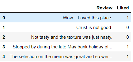
data.head()Output:
print(data.Liked.value_counts())Output:
1    500
0    500
Name: Liked, dtype: int64
In this dataset, we have two columns Review and Liked. Review is the restaurant review and Liked is the sentiment 0 and 1. 1 means the customer has liked the restaurant and 0 means not liked.
Create Wordcloud
Wordcloud is the pictorial representation of the most frequent keywords in the dataset. In a wordcloud, the font size of words is directly proportional to the frequency of the word. In order to create a wordcloud we have to first install the module wordcloud using pip command.
!pip install wordcloud Let’s create a wordcloud using wordcloud module:
# Import WordCloud and STOPWORDS
from wordcloud import WordCloud
from wordcloud import STOPWORDS
# Import matplotlib
import matplotlib.pyplot as plt


def word_cloud(text):

    # Create stopword list
    stopword_list = set(STOPWORDS)

    # Create WordCloud
    word_cloud = WordCloud(width = 550, height = 550,
                           background_color ='white',
                           stopwords = stopword_list,
                           min_font_size = 12).generate(text)

    # Set wordcloud figure size
    plt.figure(figsize = (8, 6))

    # Show image
    plt.imshow(word_cloud)

    # Remove Axis
    plt.axis("off")

    # show plot
    plt.show()

paragraph=' '.join(data.Review.tolist())
word_cloud(paragraph)
Output:
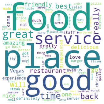
In the above word cloud, we can see that the most frequent words are food, service, place, good, great, time, restaurant, and friendly words are used.
Let’s create a word cloud for positive restaurant reviews:
paragraph=' '.join(data[data.Liked==1].Review.tolist())
word_cloud(paragraph)
Output:
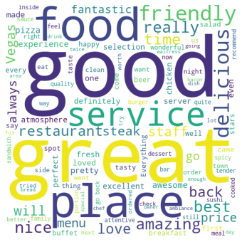
In this above word cloud, we are showing the frequent keywords of positive reviews. we can see that the most frequent words such as good, great, service, place, friendly, delicious, nice, and amazing.
paragraph=' '.join(data[data.Liked==0].Review.tolist())
word_cloud(paragraph)
Output:
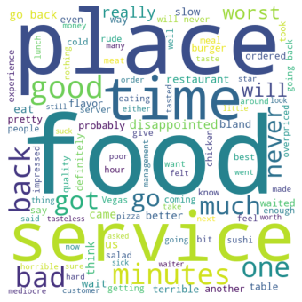
In the above word cloud, we are showing the frequent keywords of negative reviews. we can see that the most frequent words such as food, place, time, food service, bad, worst, slow, minutes, and disappointed.
Feature Generation using Bag of Words
In-Text Classification Problem, we have to generate features from the textual dataset. because we directly can’t apply the machine learning models to text data. We need to convert these text into some numbers or vectors of numbers. We are generating a Bag-of-words(BoW) for extracting features from the textual dataset. BoW converts text into the matrix of the frequency of words within a document.
# Bag of word: vectors word frequency(count)
from sklearn.feature_extraction.text import CountVectorizer

from nltk.tokenize import RegexpTokenizer

#tokenizer to remove unwanted elements from data like symbols

token = RegexpTokenizer(r'[a-zA-Z0-9]+')

cv = CountVectorizer(lowercase=True,
                     stop_words='english',
                     ngram_range = (1,1),
                     tokenizer = token.tokenize)

text_counts= cv.fit_transform(data['Review'])

print(text_counts.shape)
Output: (1000, 1834)
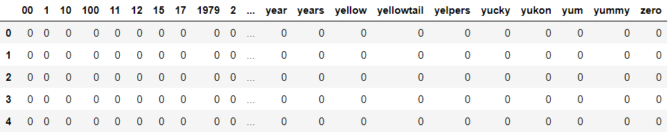
Convert CountVectorized vector into Pandas DataFrame.
count_df = pd.DataFrame(text_counts.toarray(),columns=cv.get_feature_names())
count_df.head()
Output:
Split train and test set
In order to assess the model performance, we need to split the dataset into a training set and a test set.
Let’s split dataset by using function train_test_split(). you need to pass basically 3 parameters features, target, and test_set size. Additionally, you can use random_state to select records randomly. Here, random_state simply sets seed to the random generator, so that your train-test splits are always deterministic. If you don’t set seed, it is different each time.
from sklearn.model_selection import train_test_split

X_train, X_test, y_train, y_test = train_test_split(text_counts,
                                                    data['Liked'],
                                                    test_size=0.3,
                                                    random_state=1)
Model Building and Evaluation
Let’s build the Text Classification Model using the Multinomial Naive Bayes Classifier.
First, import the MultinomialNB module and create a Multinomial Naive Bayes classifier object using MultinomialNB() function.
Then, fit your model on the train set using fit() and perform prediction on the test set using predict().
from sklearn.naive_bayes import MultinomialNB

#Import scikit-learn metrics module for accuracy calculation
from sklearn import metrics

# Model Generation Using Multinomial Naive Bayes
clf = MultinomialNB().fit(X_train, y_train)

predicted= clf.predict(X_test)

print("MultinomialNB Accuracy:",metrics.accuracy_score(y_test, predicted))
Output: MultinomialNB Accuracy: 0.7333333333333333
Well, you got a classification rate of 73.34% using BoW features, which is a good accuracy. We can still improve this performance by trying different feature engineering and classification methods.
Predict Sentiment
We can make predictions on a trained model using predict() method but before predict we must need to convert the input text into the vector using the transform() method.
# Transform into matrix
val=cv.transform(["Service of the restaurant is very slow but food was delicous"])

# make prediction
clf.predict(val)
Output: array([0], dtype=int64)
The given input review us predicted as 0 or not liked because of its slow service.
Conclusion
Congratulations, you have made it to the end of this tutorial!
In this tutorial, you have performed restaurant review sentiment analysis using text classification with the Scikit-learn library. Learn More about sentiment analysis in this article Sentiment Analysis using Python.
I look forward to hearing any feedback or questions. you can ask the question by leaving a comment and I will try my best to answer it.