Sentiment Analysis using Python
Analyze people’s sentiments and classify movie reviews
Nowadays companies want to understand, what went wrong with their latest products? what users and the general public think about the latest feature? you can quantify such information with good accuracy using sentiment analysis.
Quantifying the user’s content, idea, belief, and opinion are known as sentiment analysis. User’s online post, blogs, tweets, feedback of product helps business people to the target audience and innovate in products and services. sentiment analysis helps in understanding people in a better and more accurate way, It is not only limited to marketing, but it can also be utilized in politics, research, and security.
Human communication just not limited to words, it is more than words. Sentiments are combination words, tone, and writing style. As a data analyst, It is more important to understand our sentiments, what it really means?
There are mainly two approaches for performing sentiment analysis
- Lexicon-based: count number of positive and negative words in a given text and the larger count will be the sentiment of the text.
- Machine learning-based approach: Develop a classification model, which is trained using the prelabeled dataset of positive, negative, and neutral.
In this tutorial, you will use the second approach(Machine learning-based approach). This is how you learn sentiment and text classification with a single example.
Text Classification
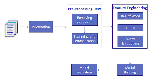
Text classification is one of the important tasks of text mining. It is a supervised approach. Identifying category or class of given text such as blog, book, web page, news articles, and tweets. It has various applications in today’s computer world such as spam detection, task categorization in CRM services, categorizing products on E-retailer websites, classifying the content of websites for a search engine, sentiments of customer feedback, etc. In the next section, you will learn how you can do text classification in python.

Performing Sentiment Analysis using Text Classification
Loading Data
Till now, you have learned data preprocessing using NLTK. Now, you will learn Text Classification. you will perform Multi-Nomial Naive Bayes Classification using scikit-learn.
In the model the building part, you can use the “Sentiment Analysis of Movie, Reviews” dataset available on Kaggle. The dataset is a tab-separated file. Dataset has four columns PhraseId, SentenceId, Phrase, and Sentiment.
This data has 5 sentiment labels:
0 — negative 1 — somewhat negative 2 — neutral 3 — somewhat positive 4 — positive
Here, you can build a model to classify the type of cultivar. The dataset is available on Kaggle, you can download it from the following link: https://www.kaggle.com/c/sentiment-analysis-on-movie-reviews/data
# Import pandas
import pandas as pd

data=pd.read_csv('train.tsv', sep='\t')

data.head()

Output:
data.info()Output: <class 'pandas.core.frame.DataFrame'> RangeIndex: 156060 entries, 0 to 156059 Data columns (total 4 columns): PhraseId 156060 non-null int64 SentenceId 156060 non-null int64 Phrase 156060 non-null object Sentiment 156060 non-null int64 dtypes: int64(3), object(1) memory usage: 4.8+ MBdata.Sentiment.value_counts()Output:2 79582 3 32927 1 27273 4 9206 0 7072 Name: Sentiment, dtype: int64
Sentiment_count=data.groupby('Sentiment').count()

plt.bar(Sentiment_count.index.values, Sentiment_count['Phrase'])

plt.xlabel('Review Sentiments')
plt.ylabel('Number of Review')

plt.show()
Feature Generation using Bag of Words
In-Text Classification Problem, we have a set of texts and their respective labels. but we directly can’t use text for our model. you need to convert these text into some numbers or vectors of numbers.
Bag-of-words model(BoW ) is the simplest way of extracting features from the text. BoW converts text into the matrix of the occurrence of words within a document. This model concerns whether given words occurred or not in the document.
Example: There are three documents:
Doc 1: I love dogs.
Doc 2: I hate dogs and knitting.
Doc 3: Knitting is my hobby and passion.
Now, you can create a matrix of documents and words by counting the occurrence of words in a given document. This matrix is known as the Document-Term Matrix(DTM).

This matrix is using a single word. It can be a combination of two or more words, which is called the bigram or trigram model and the general approach is called the n-gram model.
You can generate a document term matrix by using scikit-learn’s CountVectorizer.
from sklearn.feature_extraction.text import CountVectorizer
from nltk.tokenize import RegexpTokenizer

#tokenizer to remove unwanted elements from out data like symbols and numbers
token = RegexpTokenizer(r'[a-zA-Z0-9]+')

cv = CountVectorizer(lowercase=True,stop_words='english',ngram_range = (1,1),tokenizer = token.tokenize)

text_counts= cv.fit_transform(data['Phrase'])
Split train and test set
To understand model performance, dividing the dataset into a training set and a test set is a good strategy.
Let’s split dataset by using function train_test_split(). you need to pass basically 3 parameters features, target, and test_set size. Additionally, you can use random_state to select records randomly.
from sklearn.model_selection import train_test_split
X_train, X_test, y_train, y_test = train_test_split(text_counts, data['Sentiment'], test_size=0.3, random_state=1)
Model Building and Evaluation
Let’s build the Text Classification Model using TF-IDF.
First, import the MultinomialNB module and create Multinomial Naive Bayes classifier object using MultinomialNB() function.
Then, fit your model on the train set using fit() and perform prediction on the test set using predict().
from sklearn.naive_bayes import MultinomialNB

#Import scikit-learn metrics module for accuracy calculation
from sklearn import metrics

# Model Generation Using Multinomial Naive Bayes
clf = MultinomialNB().fit(X_train, y_train)

predicted= clf.predict(X_test)

print("MultinomialNB Accuracy:",metrics.accuracy_score(y_test, predicted))
Output: MultinomialNB Accuracy: 0.604916912299
Well, you got a classification rate of 60.49% using CountVector(or BoW), which is not considered as good accuracy. We need to improve this.
Feature Generation using TF-IDF
In Term Frequency(TF), you just count the number of words that occurred in each document. The main issue with this Term Frequency is that it will give more weight to longer documents. Term frequency is basically the output of the BoW model.
IDF(Inverse Document Frequency) measures the amount of information a given word provides across the document. IDF is the logarithmically scaled inverse ratio of the number of documents that contain the word and the total number of documents.

TF-IDF(Term Frequency-Inverse Document Frequency) normalizes the document term matrix. It is the product of TF and IDF. Word with high tf-idf in a document, it is most of the time that occurred in given documents and must be absent in the other documents. So the words must be a signature word.

from sklearn.feature_extraction.text import TfidfVectorizer

tf=TfidfVectorizer()

text_tf= tf.fit_transform(data['Phrase'])
Split train and test set (TF-IDF)
Let’s split dataset by using function train_test_split(). you need to pass basically 3 parameters features, target, and test_set size. Additionally, you can use random_state to select records randomly.
from sklearn.model_selection import train_test_split

X_train, X_test, y_train, y_test = train_test_split(text_tf, data['Sentiment'], test_size=0.3, random_state=123)
Model Building and Evaluation (TF-IDF)
Let’s build the Text Classification Model using TF-IDF.
First, import the MultinomialNB module and create Multinomial Naive Bayes classifier object using MultinomialNB() function.
Then, fit your model on the train set using fit() and perform prediction on the test set using predict().
from sklearn.naive_bayes import MultinomialNB
from sklearn import metrics

# Model Generation Using Multinomial Naive Bayes

clf = MultinomialNB().fit(X_train, y_train)
predicted= clf.predict(X_test)

print("MultinomialNB Accuracy:",metrics.accuracy_score(y_test, predicted))

Output:
MultinomialNB Accuracy: 0.586526549618
Well, you got a classification rate of 58.65% using TF-IDF features, which is not considered as good accuracy. We need to improve accuracy using some other preprocessing or feature engineering. Let’s suggest in the comment box some approach for accuracy improvement.
Conclusion
Congratulations, you have made it to the end of this tutorial!
In this tutorial, you have learned What is sentiment analysis, Feature Engineering, and text classification using scikit-learn.
I look forward to hearing any feedback or questions. you can ask the question by leaving a comment and I will try my best to answer it.
Originally published at https://www.datacamp.com/community/tutorials/text-analytics-beginners-nltk
Reach out to me on Linkedin: https://www.linkedin.com/in/avinash-navlani/