Explore Python Gensim Library For NLP

In this tutorial, we will focus on the Gensim Python library for text analysis.

Gensim is an acronym for Generate Similar. It is a free Python library for natural language processing written by Radim Rehurek which is used in word embeddings, topic modeling, and text similarity. It is developed for generating word and document vectors. It also extracts the topics from textual documents. It is an open-source, scalable, robust, fast, efficient multicore Implementation, and platform-independent.

In this tutorial, we are going to cover the following topics:

Installing Gensim

Gensim is one of the powerful libraries for natural language processing. It will support Bag of Words, TFIDF, Word2Vec, Doc2Vec, and Topic modeling. Let install the library using pip command:

pip install gensim

Create Gensim Dictionary

In this section, we will start gensim by creating a dictionary object. First, we load the text data file. you can download it from the following link.

# open the text file as an object 
file = open('hamlet.txt', encoding ='utf-8')

# read the file
text=file.read()

Now, we tokenize and preprocess the data using the string function split() and simple_preprocess() function available in gensim module.

# Tokenize data: Handling punctuations and lowercasing the text 
from gensim.utils import simple_preprocess 

# preprocess the file to get a list of tokens 
token_list =[] 

for sentence in text.split('.'):   
    # the simple_preprocess function returns a list of each sentence 
    token_list.append(simple_preprocess(sentence, deacc = True))

print (token_list[:2])

Output:

[['the', 'tragedy', 'of', 'hamlet', 'prince', 'of', 'denmark', 'by', 'william', 'shakespeare', 'dramatis', 'personae', 'claudius', 'king', 'of', 'denmark'], ['marcellus', 'officer']]

In the above code block, we have tokenized and preprocessed the hamlet text data.

• deacc (bool, optional) – Remove accent marks from tokens using deaccent() function.
• The deaccent() function is another utility function, documented at the link, which does exactly what the name and documentation suggest: removes accent marks from letters, so that, for example, ‘é’ becomes just ‘e’.
• simple_preprocess(), as per its documentation, to discard any tokens shorter than min_len=2 characters.

After tokenization and preprocessing, we will create gensim dictionary object for the above-tokenized text.

# Import gensim corpora
from gensim import corpora 

# storing the extracted tokens into the dictionary 
my_dictionary = corpora.Dictionary(token_list) 

# print the dictionary 
print(my_dictionary)

Output:

Dictionary(4593 unique tokens: ['by', 'claudius', 'denmark', 'dramatis', 'hamlet']...)

Here, gensim dictionary stores all the unique tokens.

Now, we will see how to save and load the dictionary object.

# save your dictionary to disk 
my_dictionary.save('dictionary.dict')

# load back 
load_dict = corpora.Dictionary.load('dictionary.dict')

print(load_dict)

Output:

Dictionary(4593 unique tokens: ['by', 'claudius', 'denmark', 'dramatis', 'hamlet']...)

Bag of Words

The Bag-of-words model(BoW ) is the simplest way of extracting features from the text. BoW converts text into the matrix of the occurrence of words within a document. This model concerns whether given words occurred or not in the document.

Let’s create a bag of words using function doc2bow() for each tokenized sentence. Finally, we will have a list of tokens with their frequency.

# Converting to a bag of word corpus 
BoW_corpus =[my_dictionary.doc2bow(sent, allow_update = True) for sent in token_list] 

print(BoW_corpus[:2])

[[(0, 1), (1, 1), (2, 2), (3, 1), (4, 1), (5, 1), (6, 3), (7, 1), (8, 1), (9, 1), (10, 1), (11, 1), (12, 1)], [(13, 1), (14, 1)]]

In the above code, we have generated the bag or words. In the output, you can see the index and frequency of each token. If you want to replace the index with a token then you can try the following script:

# Word weight in Bag of Words corpus 
word_weight =[] 

for doc in BoW_corpus: 
    for id, freq in doc: 
        word_weight.append([my_dictionary[id], freq]) 
        
print(word_weight[:10])

[['by', 1], ['claudius', 1], ['denmark', 2], ['dramatis', 1], ['hamlet', 1], ['king', 1], ['of', 3], ['personae', 1], ['prince', 1], ['shakespeare', 1]]

Here, you can see the list of tokens with their frequency.

TF-IDF

• In Term Frequency(TF), you just count the number of words that occurred in each document. The main issue with this Term Frequency is that it will give more weight to longer documents. Term frequency is basically the output of the BoW model.
• IDF(Inverse Document Frequency) measures the amount of information a given word provides across the document. IDF is the logarithmically scaled inverse ratio of the number of documents that contain the word and the total number of documents.
• TF-IDF(Term Frequency-Inverse Document Frequency) normalizes the document term matrix. It is the product of TF and IDF. Word with high tf-idf in a document, it is most of the time that occurred in given documents and must be absent in the other documents. 

Let’s generate the TF-IDF features for the given BoW corpus.

from gensim.models import TfidfModel
import numpy as np 

# create TF-IDF model 
tfIdf = TfidfModel(BoW_corpus, smartirs ='ntc')

# TF-IDF Word Weight 
weight_tfidf =[] 
for doc in tfIdf[BoW_corpus]: 
    for id, tf_idf in doc: 
        weight_tfidf.append([my_dictionary[id], np.around(tf_idf, decimals = 3)]) 
print(weight_tfidf[:10])

Output:
[['by', 0.146], ['claudius', 0.31], ['denmark', 0.407], ['dramatis', 0.339], ['hamlet', 0.142], ['king', 0.117], ['of', 0.241], ['personae', 0.339], ['prince', 0.272], ['shakespeare', 0.339]]

Word2Vec

Word2vec is a two-layer neural net that processes text by “vectorizing” words. Its input is a text corpus and its output is a set of vectors: feature vectors that represent words in that corpus. While Word2vec is not a deep neural network, it turns text into a numerical form that deep neural networks can understand.

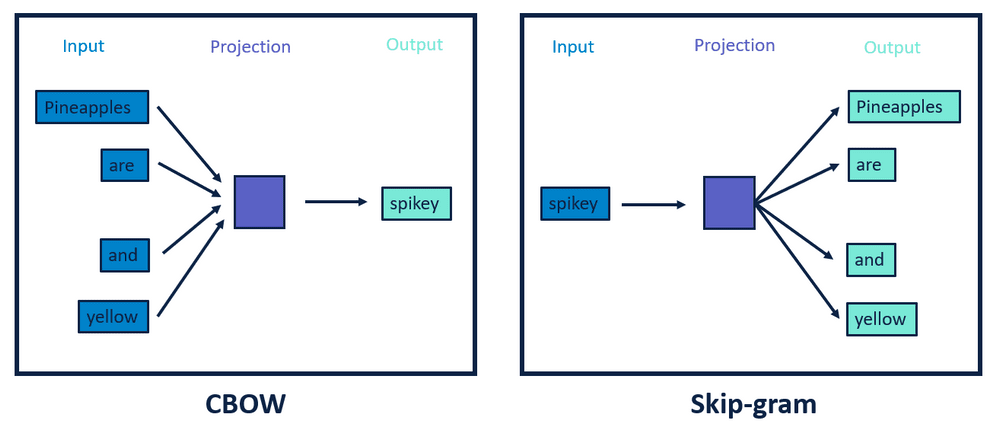
There are two main methods for woed2vec: Common Bag Of Words (CBOW) and Skip Gram.

Continuous Bag of Words (CBOW) predicts the current word based on four future and four history words. Skip-gram takes the current word as input and predicts the before and after the current word. In both types of methods, the neural network language model (NNLM) is used to train the model. Skip Gram works well with a small amount of data and is found to represent rare words well. On the other hand, CBOW is faster and has better representations for more frequent words.

Let’s implement gensim Word2Vec in python:

# import Word2Vec model
from gensim.models import Word2Vec

# Create Word2vec object
model = Word2Vec(sentences=token_list, 
                 vector_size =100, 
                 window=5, 
                 min_count=1, 
                 workers=4, 
                 sg=0) # CBOW 

#Save model
model.save("word2vec.model")

# Load trained Word2Vec model
model = Word2Vec.load("word2vec.model")

# Generate vector
vector = model.wv['think']  # returns numpy array

print(vector)

In the above code, we have built the Word2Vec model using Gensim. Here is the description for all the parameters:

• vector_size: The number of dimensions of the embeddings and the default is 100.
• min_count is for pruning the internal dictionary. Words that appear only once or twice in a billion-word corpus are probably uninteresting typos and garbage.
• workers , the last of the major parameters (full list here) is for training parallelization.
• window: Maximum distance between the current and predicted word within a sentence.
• sg: stands for skip-gram; 0- CBOW and 1:skipgram

Output:
[-0.27096474 -0.02201273  0.04375215  0.16169178  0.385864   -0.00830234
  0.06216158 -0.14317605  0.17866768  0.13853565 -0.05782828 -0.24181016
 -0.21526945 -0.34448552 -0.03946546  0.25111085  0.03826794 -0.31459117
  0.05657561 -0.10587984  0.0904238  -0.1054946  -0.30354315 -0.12670684
 -0.07937846 -0.09390186  0.01288407 -0.14465155  0.00734721  0.21977565
  0.09089493  0.27880424 -0.12895903  0.03735492 -0.36632115  0.07415111
  0.10245194 -0.25479802  0.04779665 -0.06959599  0.05201627 -0.08305986
 -0.00901385  0.01109841  0.03884205  0.2771041  -0.17801927 -0.17918047
  0.1551789  -0.04730623 -0.15239601  0.09148847 -0.16169599  0.07088429
 -0.07817879  0.19048482  0.2557149  -0.2415944   0.17011274  0.11839501
  0.1798175   0.05671703  0.03197689  0.27572715 -0.02063731 -0.04384637
 -0.08028547  0.08083986 -0.3160063  -0.01283481  0.24992462 -0.04269576
 -0.03815364  0.08519065  0.02496272 -0.07471556  0.17814435  0.1060199
 -0.00525795 -0.08447327  0.09727245  0.01954588  0.055328    0.04693184
 -0.04976451 -0.15165417 -0.19015886  0.16772328  0.02999189 -0.05189768
 -0.0589773   0.07928728 -0.29813886  0.05149718 -0.14381753 -0.15011951
  0.1745079  -0.14101334 -0.20089763 -0.13244842]

Lets find most similar words for a given word:

# Finding most similar words
model.wv.most_similar('flash')

Output:
[('natural', 0.9266888499259949),
 ('visage', 0.9253427982330322),
 ('yea', 0.9249608516693115),
 ('pyrrhus', 0.9225320816040039),
 ('osric', 0.9224336743354797),
 ('honest', 0.9221916198730469),
 ('fly', 0.9220262169837952),
 ('work', 0.9218302369117737),
 ('woman', 0.9209260940551758),
 ('once', 0.9208680391311646)]

Pretrained Word2Vec: Google’s Word2Vec, Standford’s Glove and Fasttext

• Google’s Word2Vec treats each word in the corpus like an atomic entity and generates a vector for each word. In this sense Word2vec is very much like Glove – both treat words as the smallest unit to train on. 
• Google’s Word2Vec is a “predictive” model that predicts the context given word, GLOVE learns by factorizing a co-occurrence matrix.
• Fasttext treats each word as composed of character ngrams. So the vector for a word is made of the sum of this character n-grams. 
• Google’s Word2vec and GLOVE do not solve the problem of out-of-vocabulary words (or generalization to unknown words) but Fasttext can solve this problem because it’s based on each character n grams.
• The biggest benefit of using FastText is that it generates better word embeddings for rare words, or even words not seen during training because the n-gram character vectors are shared with other words. 

Google’s Word2Vec

In this section, we will see how Google’s pre-trained Word2Vec model can be used in Python. We are using here gensim package for an interface to word2vec. This model is trained on the vocabulary of 3 million words and phrases from 100 billion words of the Google News dataset. The vector length for each word is 300. You can download Google’s pre-trained model here.

Let’s load Google’s pre-trained model and print the shape of the vector:

from gensim.models.word2vec import Word2Vec
from gensim.models import KeyedVectors

model = KeyedVectors.load_word2vec_format('GoogleNews-vectors-negative300.bin', binary=True)

print(model.wv['reforms'].shape)

Output: (300,)

Standford Glove

GloVe stands for Global Vectors for Word Representation. It is an unsupervised learning algorithm for generating vector representations for words. You can read more about Glove in this research paper. It is a new global log-bilinear regression model for the unsupervised learning of word representations. You can use the following list of models trained on the Twitter dataset:

• glove-twitter-25 (104 MB)
• glove-twitter-50 (199 MB)
• glove-twitter-100 (387 MB)
• glove-twitter-200 (758 MB)

import gensim.downloader as api

# Download the model and return as object ready for use
model_glove_twitter = api.load("glove-twitter-25")

# Print shape of the vector
print(model_glove_twitter['reforms'].shape)

# Print vector for word 'reform' 
print(model_glove_twitter['reforms'])

Output:
(25,)
[ 0.37207    0.91542   -1.6257    -0.15803    0.38455   -1.3252
 -0.74057   -2.095      1.0401    -0.0027519  0.33633   -0.085222
 -2.1703     0.91529    0.77599   -0.87018   -0.97346    0.68114
  0.71777   -0.99392    0.028837   0.24823   -0.50573   -0.44954
 -0.52987  ]

# get similar items
model_glove_twitter.most_similar("policies",topn=10)

Output:
[('policy', 0.9484813213348389),
 ('reforms', 0.9403933882713318),
 ('laws', 0.94012051820755),
 ('government', 0.9230710864067078),
 ('regulations', 0.9168934226036072),
 ('economy', 0.9110006093978882),
 ('immigration', 0.9105909466743469),
 ('legislation', 0.9089651107788086),
 ('govt', 0.9054746627807617),
 ('regulation', 0.9050778746604919)]

Facebook FastText

FastText is an improvement in the Word2Vec model that is proposed by Facebook in 2016. FastText spits the words into n-gram characters instead of using the individual word. It uses the Neural Network to train the model. The core advantage of this technique is that can easily represent the rare words because some of their n-grams may also appear in other trained words. Let’s see how to use FastText with Gensim in the following section.

 Import FastText 
from gensim.models import FastText

# Create FastText Model object
model = FastText(vector_size=25, window=3, min_count=1)  # instantiate

# Build Vocab
model.build_vocab(corpus_iterable=token_list)

# Train FastText model
model.train(corpus_iterable=token_list, total_examples=len(token_list), epochs=10)  # train

model.wv['policy']

Output:
array([-0.328225  ,  0.2092654 ,  0.09407859, -0.08436475, -0.18087168,
       -0.19953477, -0.3864786 ,  0.08250062,  0.08613443, -0.14634965,
        0.18207662,  0.20164935,  0.32687476,  0.05913997, -0.04142053,
        0.01215196,  0.07229924, -0.3253025 , -0.15895212,  0.07037129,
       -0.02852136,  0.01954574, -0.04170248, -0.08522341,  0.06419735,
       -0.16668107,  0.11975338, -0.00493952,  0.0261423 , -0.07769344,
       -0.20510232, -0.05951802, -0.3080587 , -0.13712431,  0.18453395,
        0.06305533, -0.14400929, -0.07675331,  0.03025392,  0.34340212,
       -0.10817952,  0.25738955,  0.00591787, -0.04097764,  0.11635819,
       -0.634932  , -0.367688  , -0.19727138, -0.1194628 ,  0.00743668],
      dtype=float32)

# Finding most similar words
model.wv.most_similar('present')

Output:
[('presentment', 0.999993622303009),
 ('presently', 0.9999920725822449),
 ('moment', 0.9999914169311523),
 ('presence', 0.9999902248382568),
 ('sent', 0.999988317489624),
 ('whose', 0.9999880194664001),
 ('bent', 0.9999875426292419),
 ('element', 0.9999874234199524),
 ('precedent', 0.9999873042106628),
 ('gent', 0.9999872446060181)]

Doc2Vec

Doc2vec is used to represent documents in the form of a vector. It is based on the generalized approach of the Word2Vec method. In order to deep dive into doc2vec, First, you should understand how to generate word to vectors (word2vec). Doc2Vec is used to predict the next word from numerous sample contexts of the original paragraph. It addresses the semantics of the text.

• In Distributed Memory Model of Paragraph Vectors (PV-DM), paragraph tokens remember the missing context in the paragraph. It is like a continuous bag-of-words (CBOW) version of Word2Vec.
• Distributed Bag of Words version of Paragraph Vector (PV-DBOW) ignores the context of input words and predicts missing words from a random sample. It is like the Skip-Gram version of Word2vec

documents=text.split(".")

documents[:5]

from collections import namedtuple

# Transform data (you can add more data preprocessing steps) 
docs = []
analyzedDocument = namedtuple('AnalyzedDocument', 'words tags')
for i, text in enumerate(documents):
    words = text.lower().split()
    tags = [i]
    docs.append(analyzedDocument(words, tags))

print(docs[:2])

Output:
[AnalyzedDocument(words=['the', 'tragedy', 'of', 'hamlet,', 'prince', 'of', 'denmark', 'by', 'william', 'shakespeare', 'dramatis', 'personae', 'claudius,', 'king', 'of', 'denmark'], tags=[0]), AnalyzedDocument(words=['marcellus,', 'officer'], tags=[1])]

In the above code block, first, we create the document using namedtuple collection. NamedTuple is used to create a lightweight data structure similar to a class without defining its details. You can also say it is like dictionaries, which contain keys and values. After this, let’s create a model for Doc2Vec:

from gensim.models import doc2vec

model = doc2vec.Doc2Vec(docs,
                        vector_size=100,
                        window=5, 
                        min_count=1, 
                        workers=4,
                        dm=0) # PV-DBOW

vector=model.infer_vector(['the', 'tragedy', 'of', 'hamlet,', 'prince', 'of', 'denmark', 'by', 'william', 
                    'shakespeare', 'dramatis', 'personae', 'claudius,', 'king', 'of', 'denmark'])

print(vector)

Output:
[-1.5818793e-02  1.3085594e-02 -1.1896869e-02 -3.0695410e-03
  1.5006907e-03 -1.3316960e-02 -5.6281965e-03  3.1253812e-03
 -4.0207659e-03 -9.0181744e-03  1.2115648e-02 -1.2316694e-02
  9.3884282e-03 -1.2136344e-02  9.3199247e-03  6.0257949e-03
 -1.1087678e-02 -1.6263386e-02  3.0145817e-03  9.2168162e-03
 -3.1892660e-03  2.5632046e-03  4.1057081e-03 -1.1103139e-02
 -4.4368235e-03  9.3003511e-03 -1.9984354e-05  4.6007405e-03
  4.5250896e-03  1.4299035e-02  6.4971978e-03  1.3330076e-02
  1.6638277e-02 -8.3673699e-03  1.4617097e-03 -8.7684026e-04
 -5.3776056e-04  1.2898060e-02  5.5408065e-04  6.9614425e-03
  2.9868495e-03 -1.3385005e-03 -3.4805303e-03  1.0777158e-02
 -1.1053825e-02 -8.0987150e-03  3.1651056e-03 -3.6159047e-04
 -3.0776947e-03  4.9342304e-03 -1.1290920e-03 -4.8262491e-03
 -9.2841331e-03 -1.4540913e-03 -1.0785381e-02 -1.7799810e-02
  3.4300602e-04  2.4301475e-03  6.0869306e-03 -4.3078070e-03
  2.9106432e-04  1.3333942e-03 -7.1321065e-03  4.3218113e-03
  7.5919051e-03  1.7675487e-03  1.9759729e-03 -1.6749580e-03
  2.5316922e-03 -7.4808724e-04 -7.0081712e-03 -7.2277770e-03
  2.1022926e-03 -7.2621077e-04  1.6523260e-03  7.7043297e-03
  4.9248277e-03  9.8303892e-03  4.2252508e-03  3.9137071e-03
 -6.4144642e-03 -1.5699258e-03  1.5538614e-02 -1.8792158e-03
 -2.2203794e-03  6.2514015e-04  9.6203719e-04 -1.5944529e-02
 -1.8801112e-03 -2.8503922e-04 -4.4923062e-03  8.4128296e-03
 -2.0803667e-03  1.6383808e-02 -1.6173380e-04  3.9917473e-03
  1.2395959e-02  9.2958640e-03 -1.7370760e-03 -4.5007761e-04]

In the above code, we have built the Doc2Vec model using Gensim. Here is the description for all the parameters:

• dm ({1,0}, optional) – Defines the training algorithm. If dm=1, ‘distributed memory’ (PV-DM) is used. Otherwise, distributed bag of words (PV-DBOW) is employed.
• vector_size (int, optional) – Dimensionality of the feature vectors.
• window (int, optional) – The maximum distance between the current and predicted word within a sentence.
• alpha (float, optional) – The initial learning rat

Summary

Congratulations, you have made it to the end of this tutorial!

In this article, we have learned Gensim Dictionary, Bag of Words, TFIDF, Word2Vec, and Doc2Vec. We have also focused on Google’s Word2vec, Standford’s Glove, and Facebook’s FastText. We have performed all the experiments using gensim library. Of course, this is just the beginning, and there’s a lot more that we can do using Gensim in natural language processing. You can check out this article on Topic modeling.