KNN Classification using Scikit-learn
Learn K-Nearest Neighbor(KNN) Classification and build a KNN classifier using Python Scikit-learn package.
K Nearest Neighbor(KNN) is a very simple, easy-to-understand, versatile, and one of the topmost machine learning algorithms. KNN used in a variety of applications such as finance, healthcare, political science, handwriting detection, image recognition, and video recognition. In Credit ratings, financial institutes will predict the credit rating of customers. In loan disbursement, banking institutes will predict whether the loan is safe or risky. In political science, classifying potential voters in two classes will vote or won’t vote. KNN algorithm used for both classification and regression problems. KNN algorithm based on the feature similarity approach.
In this tutorial, you are going to cover the following topics:
- K-Nearest Neighbor Algorithm
- How does the KNN algorithm work?
- Eager Vs Lazy learners
- How do you decide the number of neighbors in KNN?
- Curse of Dimensionality
- Classifier Building in Scikit-learn
- Pros and Cons
- How to improve KNN performance?
- Conclusion
K-Nearest Neighbors
KNN is a non-parametric and lazy learning algorithm. Non-parametric means there is no assumption for underlying data distribution. In other words, the model structure determined from the dataset. This will be very helpful in practice where most of the real-world datasets do not follow mathematical theoretical assumptions. The lazy algorithm means it does not need any training data points for model generation. All training data used in the testing phase. This makes training faster and the testing phase slower and costlier. The costly testing phase means time and memory. In the worst case, KNN needs more time to scan all data points, and scanning all data points will require more memory for storing training data.
For more such tutorials, projects, and courses visit DataCamp:
How does the KNN algorithm work?
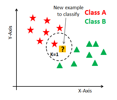
In KNN, K is the number of nearest neighbors. The number of neighbors is the core deciding factor. K is generally an odd number if the number of classes is 2. When K=1, then the algorithm is known as the nearest neighbor algorithm. This is the simplest case. Suppose P1 is the point, for which label needs to predict. First, you find the closest point to P1 and then the label of the nearest point assigned to P1.
Suppose P1 is the point, for which label needs to predict. First, you find the k closest point to P1 and then classify points by majority vote of its k neighbors. Each object votes for their class and the class with the most votes is taken as the prediction. For finding closest similar points, you find the distance between points using distance measures such as Euclidean distance, Hamming distance, Manhattan distance, and Minkowski distance. KNN has the following basic steps:
- Calculate distance
- Find closest neighbors
- Vote for labels

Eager Vs. Lazy Learners
Eager learners mean when given training points will construct a generalized model before performing prediction on given new points to classify. You can think of such learners as being ready, active, and eager to classify unobserved data points.
Lazy Learning means there is no need for learning or training of the model and all of the data points used at the time of prediction. Lazy learners wait until the last minute before classifying any data point. Lazy learners stores merely the training dataset and waits until classification needs to perform. Only when it sees the test tuple does it perform generalization to classify the tuple based on its similarity to the stored training tuples. Unlike eager learning methods, lazy learners do less work in the training phase and more work in the testing phase to make a classification. Lazy learners are also known as instance-based learners because lazy learners store the training points or instances, and all learning is based on instances.
Curse of Dimensionality
KNN performs better with a lower number of features than a large number of features. You can say that when the number of features increases than it requires more data. An increase in dimension also leads to the problem of overfitting. To avoid overfitting, the needed data will need to grow exponentially as you increase the number of dimensions. This problem of higher dimension is known as the Curse of Dimensionality.
To deal with the problem of the curse of dimensionality, you need to perform principal component analysis before applying any machine learning algorithm, or you can also use the feature selection approach. Research has shown that in large dimensions Euclidean distance is not useful anymore. Therefore, you can prefer other measures such as cosine similarity, which get decidedly less affected by a high dimension.
How do you decide the number of neighbors in KNN?
Now, you understand the KNN algorithm working mechanism. At this point, the question arises that How to choose the optimal number of neighbors? And what are its effects on the classifier? The number of neighbors(K) in KNN is a hyperparameter that you need to choose at the time of model building. You can think of K as a controlling variable for the prediction model.
Research has shown that no optimal number of neighbors suits all kinds of data sets. Each dataset has its own requirements. In the case of a small number of neighbors, the noise will have a higher influence on the result, and a large number of neighbors make it computationally expensive. Research has also shown that a small number of neighbors are the most flexible fit which will have low bias but the high variance and a large number of neighbors will have a smoother decision boundary which means lower variance but higher bias.
Generally, Data scientists choose an odd number if the number of classes is even. You can also check by generating the model on different values of k and check their performance. You can also try the Elbow method here.

Building KNN Classifier in Scikit-learn
Defining dataset
Let’s first create your own dataset. Here you need two kinds of attributes or columns in your data: Feature and label. The reason for the two types of columns is the “supervised nature of KNN algorithm”.
# Assigning features and label variables
# First Feature
weather=['Sunny','Sunny','Overcast','Rainy','Rainy','Rainy','Overcast','Sunny','Sunny',
'Rainy','Sunny','Overcast','Overcast','Rainy']
# Second Feature
temp=['Hot','Hot','Hot','Mild','Cool','Cool','Cool','Mild','Cool','Mild','Mild','Mild','Hot','Mild']# Label or target varible
play=['No','No','Yes','Yes','Yes','No','Yes','No','Yes','Yes','Yes','Yes','Yes','No']
In this dataset, you have two features (weather and temperature) and one label(play).
Encoding data columns
Various machine learning algorithms require numerical input data, so you need to represent categorical columns in a numerical column.
In order to encode this data, you could map each value to a number. e.g. Overcast:0, Rainy:1, and Sunny:2.
This process is known as label encoding, and sklearn conveniently will do this for you using Label Encoder.
# Import LabelEncoder
from sklearn import preprocessing

#creating labelEncoder
le = preprocessing.LabelEncoder()

# Converting string labels into numbers.
weather_encoded=le.fit_transform(weather)
print(weather_encoded)
Output: [2 2 0 1 1 1 0 2 2 1 2 0 0 1]
Here, you imported the preprocessing module and created the Label Encoder object. Using this LabelEncoder object, you can fit and transform the “weather” column into the numeric column.
Similarly, you can encode temperature and label it into numeric columns.
# converting string labels into numbers
temp_encoded=le.fit_transform(temp)

label=le.fit_transform(play)
Combining Features
Here, you will combine multiple columns or features into a single set of data using “zip” function
#combinig weather and temp into single listof tuples
features=list(zip(weather_encoded,temp_encoded))
Generating Model
Let’s build the KNN classifier model.
First, import the KNeighborsClassifier module and create a KNN classifier object by passing the argument number of neighbors in KNeighborsClassifier() function.
Then, fit your model on the train set using fit() and perform prediction on the test set using predict().
from sklearn.neighbors import KNeighborsClassifier

# Create KNN Classifier
model = KNeighborsClassifier(n_neighbors=3)

# Train the model using the training sets
model.fit(features,label)

#Predict Output
predicted= model.predict([[0,2]])

# 0:Overcast, 2:Mild
print(predicted)
Output: [1]
In the above example, you have given input [0,2], where 0 means Overcast weather and 2 means Mild temperature. The model predicts [1], which means play.
KNN with Multiple Labels
Till now, you have learned How to create a KNN classifier for two in python using scikit-learn. Now you will learn about KNN with multiple classes.
In the model the building part, you can use the wine dataset, which is a very famous multi-class classification problem. This data is the result of a chemical analysis of wines grown in the same region in Italy using three different cultivars. The analysis determined the quantities of 13 constituents found in each of the three types of wines.
The dataset comprises 13 features (‘alcohol’, ‘malic_acid’, ‘ash’, ‘alcalinity_of_ash’, ‘magnesium’, ‘total_phenols’, ‘flavanoids’, ‘nonflavanoid_phenols’, ‘proanthocyanins’, ‘color_intensity’, ‘hue’, ‘od280/od315_of_diluted_wines’, ‘proline’) and a target (type of cultivars).
This data has three types of cultivar classes: ‘class_0’, ‘class_1’, and ‘class_2’. Here, you can build a model to classify the type of cultivar. The dataset is available in the scikit-learn library, or you can also download it from the UCI Machine Learning Library.
Loading Data
Let’s first load the required wine dataset from scikit-learn datasets.
#Import scikit-learn dataset library
from sklearn import datasets#Load dataset
wine = datasets.load_wine()
Exploring Data
After you have loaded the dataset, you might want to know a little bit more about it. You can check features and target names.
# print the names of the features
print(wine.feature_names)

# print the label species(class_0, class_1, class_2)
print(wine.target_names)
Output: ['alcohol', 'malic_acid', 'ash', 'alcalinity_of_ash', 'magnesium', 'total_phenols', 'flavanoids', 'nonflavanoid_phenols', 'proanthocyanins', 'color_intensity', 'hue', 'od280/od315_of_diluted_wines', 'proline'] ['class_0' 'class_1' 'class_2']
Let’s check top 5 records of the feature set.
# print the wine data (top 5 records)
print(wine.data[0:5])
Output:
[[  1.42300000e+01   1.71000000e+00   2.43000000e+00   1.56000000e+01
    1.27000000e+02   2.80000000e+00   3.06000000e+00   2.80000000e-01
    2.29000000e+00   5.64000000e+00   1.04000000e+00   3.92000000e+00
    1.06500000e+03]
 [  1.32000000e+01   1.78000000e+00   2.14000000e+00   1.12000000e+01
    1.00000000e+02   2.65000000e+00   2.76000000e+00   2.60000000e-01
    1.28000000e+00   4.38000000e+00   1.05000000e+00   3.40000000e+00
    1.05000000e+03]
 [  1.31600000e+01   2.36000000e+00   2.67000000e+00   1.86000000e+01
    1.01000000e+02   2.80000000e+00   3.24000000e+00   3.00000000e-01
    2.81000000e+00   5.68000000e+00   1.03000000e+00   3.17000000e+00
    1.18500000e+03]
 [  1.43700000e+01   1.95000000e+00   2.50000000e+00   1.68000000e+01
    1.13000000e+02   3.85000000e+00   3.49000000e+00   2.40000000e-01
    2.18000000e+00   7.80000000e+00   8.60000000e-01   3.45000000e+00
    1.48000000e+03]
 [  1.32400000e+01   2.59000000e+00   2.87000000e+00   2.10000000e+01
    1.18000000e+02   2.80000000e+00   2.69000000e+00   3.90000000e-01
    1.82000000e+00   4.32000000e+00   1.04000000e+00   2.93000000e+00
    7.35000000e+02]]
Let’s check the records of the target set.
# print the wine labels (0:Class_0, 1:Class_1, 2:Class_3)
print(wine.target)
Output: [0 0 0 0 0 0 0 0 0 0 0 0 0 0 0 0 0 0 0 0 0 0 0 0 0 0 0 0 0 0 0 0 0 0 0 0 0 0 0 0 0 0 0 0 0 0 0 0 0 0 0 0 0 0 0 0 0 0 0 1 1 1 1 1 1 1 1 1 1 1 1 1 1 1 1 1 1 1 1 1 1 1 1 1 1 1 1 1 1 1 1 1 1 1 1 1 1 1 1 1 1 1 1 1 1 1 1 1 1 1 1 1 1 1 1 1 1 1 1 1 1 1 1 1 1 1 1 1 1 1 2 2 2 2 2 2 2 2 2 2 2 2 2 2 2 2 2 2 2 2 2 2 2 2 2 2 2 2 2 2 2 2 2 2 2 2 2 2 2 2 2 2 2 2 2 2 2 2]
Let’s explore it for a bit more. You can also check the shape of the dataset using shape.
# print data(feature)shape
print(wine.data.shape)

# print target(or label)shape
print(wine.target.shape)
(178, 13) (178,)
Splitting Data
To understand model performance, dividing the dataset into a training set and a test set is a good strategy.
Let’s split dataset by using function train_test_split(). You need to pass 3 parameters features, target, and test_set size. Additionally, you can use random_state to select records randomly.
# Import train_test_split function
from sklearn.model_selection import train_test_split

# Split the dataset into training set and test set
X_train, X_test, y_train, y_test = train_test_split(wine.data, wine.target, test_size=0.3) # 70% training and 30% test
Generating Model for K=5
Let’s build the KNN classifier model for k=5.
#Import knearest neighbors Classifier model
from sklearn.neighbors import KNeighborsClassifier

# Create KNN Classifier
knn = KNeighborsClassifier(n_neighbors=5)

# Train the model using the training sets
knn.fit(X_train, y_train)

# Predict the response for test dataset
y_pred = knn.predict(X_test)
Model Evaluation for k=5
Let’s estimate, how accurately the classifier or model can predict the type of cultivars.
Accuracy can be computed by comparing actual test set values and predicted values.
#Import scikit-learn metrics module for accuracy calculation
from sklearn import metrics

# Model Accuracy, how often is the classifier correct?
print("Accuracy:",metrics.accuracy_score(y_test, y_pred))
Output: Accuracy: 0.685185185185
Well, you got a classification rate of 68.51%, considered as good accuracy.
For further evaluation, you can also create a model for a different number of neighbors.
Re-generating Model for K=7
Let’s build the KNN classifier model for k=7.
#Import knearest neighbors Classifier model
from sklearn.neighbors import KNeighborsClassifier

#Create KNN Classifier
knn = KNeighborsClassifier(n_neighbors=7)

#Train the model using the training sets
knn.fit(X_train, y_train)

#Predict the response for test dataset
y_pred = knn.predict(X_test)
Model Evaluation for k=7
Let’s again estimate, how accurately the classifier or model can predict the type of cultivars for k=7.
#Import scikit-learn metrics module for accuracy calculation
from sklearn import metrics

# Model Accuracy, how often is the classifier correct?
print("Accuracy:",metrics.accuracy_score(y_test, y_pred))
Output: Accuracy: 0.777777777778
Well, you got a classification rate of 77.77%, considered as good accuracy.
Here, you have increased the number of neighbors in the model, and accuracy got increased. But, this is not necessary for each case that an increase in many neighbors increases the accuracy. For a more detailed understanding of it, you can refer to the section “How to decide the number of neighbors?” of this tutorial.
Pros
The training phase of K-nearest neighbor classification is much faster compared to other classification algorithms. There is no need to train a model for generalization, That is why KNN is known as the simple and instance-based learning algorithm. KNN can be useful in case of nonlinear data. It can be used with the regression problem. Output value for the object is computed by the average of k closest neighbors value.
Cons
The testing phase of K-nearest neighbor classification is slower and costlier in terms of time and memory. It requires large memory for storing the entire training dataset for prediction. KNN requires the scaling of data because KNN uses the Euclidean distance between two data points to find the nearest neighbors. Euclidean distance is sensitive to magnitudes. The features with high magnitudes will weigh more than features with low magnitudes. KNN also not suitable for large dimensional data.
How to improve KNN?
For better results, normalizing data on the same scale is highly recommended. Generally, the normalization range considered between 0 and 1. KNN is not suitable for large dimensional data. In such cases, the dimension needs to reduce to improve performance. Also, handling missing values will help us in improving results.
Conclusion
Congratulations, you have made it to the end of this tutorial!
In this tutorial, you have learned the K-Nearest Neighbor algorithm; it’s working, eager and lazy learner, the curse of dimensionality, model building, and evaluation on wine dataset using Python Scikit-learn package. Also, discussed its advantages, disadvantages, and performance improvement suggestions.
I look forward to hearing any feedback or questions. You can ask questions by leaving a comment, and I will try my best to answer it.
Originally published at https://www.datacamp.com/community/tutorials/k-nearest-neighbor-classification-scikit-learn
Do you want to learn data science, check out on DataCamp.
For more such article, you can visit my blog Machine Learning Geek
Reach out to me on Linkedin: https://www.linkedin.com/in/avinash-navlani/