SVMs with Julia

We’re almost at the end of another month of Julia here on MachineLearningGeek, and we’ll be quickly covering Support Vector Machines today.

Today we’ll be showcasing another machine learning library for Julia. Much like in Python you’d use SciKitLearn for simple algorithms like an SVM, while you’d use PyTorch or the likes for neural networks. We have MLJ.jl for simpler algorithms, while Flux.jl is reserved for neural networks. (There’s also MLJFlux for when you want to put both of them together). So lets get started.

As is the custom, we first import the packages we’ll be needing later, MLJ will be our workhorse, and Gafly we’ll use for plotting.

using MLJ
import RDatasets: dataset
using Gadfly

I prefer to use random values while learning, and so I define a function to initiate my variables like that:

function init()
	X = randn(40, 2)
	y = vcat(-ones(20), ones(20))
	return X,y
	end

	X,y=init()

Today we’re going to use a slightly different way of starting off our data, we’ll use y as a mask:

ym1 = y .== -1
ym2 = .!ym1

And then plot our data

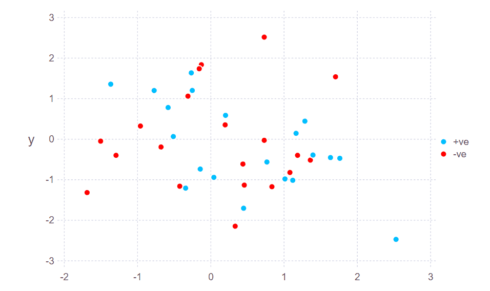
plot(
layer(x=X[ym1, 1], y=X[ym1, 2], ),
layer(x=X[ym2, 1], y=X[ym2, 2], Theme(default_color=colorant"red")),
 #Scale.shape_discrete(levels=["+ve","-ve"]),
 Guide.manual_color_key("", ["+ve", "-ve"], ["deepskyblue","red"]),
	point_shapes=[Shape.circle, Shape.star1])

The reason we constructed our data in such a convoluted way was that in order to use our data with MLJ, we’re going to have to put it in a format that MLJ likes. So, now we do that by converting into tables:

tX = MLJ.table(X)
ty = categorical(y);

Finally, we do the modelling. So, you should know that just like Plots.jl, MLJ.jl, instead of writing everything from scratch, relies on pre-existing libraries. For SVMs, that pre-existing library is LIBSVM, which is pretty standard. So, we load it using the load macro provided by MLJ:

@load SVC pkg=LIBSVM

Then we instantiate it and feed the data:

svc_mdl = SVC()
svc = machine(svc_mdl, tX, ty)

To fit the data is as simple as:

fit!(svc);

And we can check the accuracy of our model by using the misclassification_rate function provided by MLJ

ypred = predict(svc, tX)
misclassification_rate(ypred, ty)

And you can see that even on random data, we get a 0.1 accuracy. That’s pretty good! You can check out the Pluto notebook at the following link:

https://github.com/mathmetal/Misc/blob/master/MLG/SimpleSVM.jl