Measures of Dispersion

To understand the data well, only studying measures of central tendency is not enough. One essential measure is how the data is scattered or dispersed. Measures of dispersion indicate how the data is spread or scattered from the measures of central tendency. Measures Of dispersion are also known as “Measures of Variability” because they indicate the variability of the data and how much we still do not know about the data.

In this blog, we will discuss four commonly used measures of dispersion.

1. Range
2. Inter-quartile range (IQR)
3. Variance
4. Standard deviation

Range

The simplest measure of dispersion is Range; it is the difference between the highest value and lowest value in the dataset. It offers a crude insight into the spread of the data but is very susceptible to outliers. The range is helpful when you want to focus on extreme values in the dataset. The formula of Range is:

Range = Highest value – lowest value

Let’s understand with an example of a weather report, the temperature is measured every three hours during a given day.

Hour	Temperature
0.00	12⁰C
3.00	6⁰C
6.00	9⁰C
9.00	15⁰C
12.00	20⁰C
15.00	27⁰C
18.00	18⁰C
21.00	16⁰C
0.00	13⁰C

As the table shows the temperature which is measured every three hours, the green highlighted row shows the minimum value for the temperature was 6 ⁰C at 3.00 hours and the red highlighted row shows the maximum value for the temperature was 27 ⁰C at 15.00 hours. This temperature is an important measure when the temperature is one of the deciding factors for open-air events.

Inter-Quartile Range

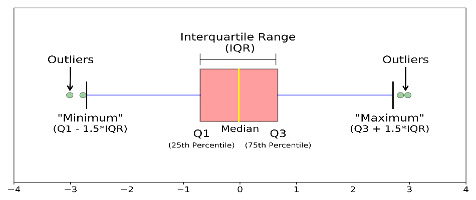
The interquartile range is a measure of dispersion, as it also measures the variability of the data, IQR indicates how the data in a series is dispersed from the mean. It measures the difference between the third quartile and the first quartile of the data. It means IQR measures the spread of the middle 50% of the dataset. As the IQR goes up the data points are more spread out and if the IQR is small the assumed-to-be data is spread around the mean. IQR is also very helpful to determine the outlier in the datasets. To calculate IQR first we have to sort the data in ascending order.

The Formula of IQR is:

IQR = Third Quartile – First Quartile

Let’s understand how to find the interquartile range:

Suppose we have a data series 88,89,89,89,90,91,91,91,92

So, to find out the IQR first we have to sort the data in ascending order as the data is already sorted so we don’t need to sort it. Now next find the median (middle value) of the data this is identified as Q2, and the middle value of the dataset is 90.

88,89,89,89,90,91,91,91,92

As the dataset is divided into two parts, now find the middle value of the first half which is identified as Q1 89, and the second half which is identified as Q3 is 91.

So, the IQR is – = 91-89= 2

Visualization of interquartile range through box-plot:

We used IQR when we were more interested in middle value and less interested in extremes.

Variance

Variance is one of the important measures of dispersion, Variance measures the variability of the data around its mean or average. In other words, variance indicates how the data is deviated or dispersed from its mean or average. High variance means there is more variability or we can say that the data deviates more from its mean whereas low variance means there is less variability. If the variance is zero that means all the values in the data are identical. Variance can never be negative. It is denoted by (sigma square).

The formula for population variance:

where N is the population size and X are data points and μ is the population mean.

The formula for sample variance:

where n is the sample size and X are the data points and x̄ (X-bar) is the sample mean.

Let’s understand variance with an example

Suppose I am traveling from Indore to Bhopal by car, my car speed data is 0,30,60,50,80,100 the average speed of the car is 53.33. Now we calculate the variance of car speed data, we get the variance of 1055.55(by population formula). As we see variance is too far from its average which indicates our variance is too high which means my car speed is fluctuating a lot. So in conclusion, we say that the driver driving a car roughly means he is not a good driver because the car speed data varies a lot.

Standard Deviation

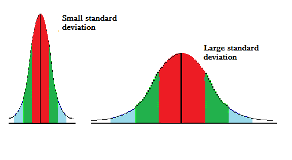
Standard deviation is an important measure of dispersion and is frequently used in statistics. Standard deviation is simply the square root of variance. It indicates how far away the dispersion of the dataset is from its mean. It is denoted by (sigma). Simply standard deviation helps us find the data’s spread about its mean or average. A low Standard deviation indicates that the data are less spread from their average whereas a high standard deviation indicates the data are more spread out from its average.

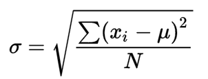
The formula of standard deviation for population:

where N is the population size and X is the data points and μ is the sample mean.

The formula of standard deviation for the sample:

where n is the sample size, X is the data points, and x̄ (X-bar) is the sample mean.

Let’s take the above example of car speed data, the variance is 1055.55, we calculate the standard deviation which is 32.48, so this indicates that our data fluctuates between 53.33 ± 32.48 (if take one standard deviation, that is 68% of the total data).

In financial risk management, investors often worry about the volatility of return i.e. how much the return spreads from the average. Standard deviation helps to provide a measure of the volatility of return and is considered to be a very important measure of risk.

Summary

In this tutorial, we have discussed the measures of dispersion or measures of variability. we have discussed the Range, Interquartile range (IQR), Variance, and Standard deviation with a real-life example.