In this tutorial, you’ll learn the basics of factor analysis and how to implement it in Python.

Factor Analysis (FA) is an exploratory data analysis method used to search influential underlying factors or latent variables from a set of observed variables. It helps in data interpretations by reducing the number of variables. It extracts maximum common variance from all variables and puts them into a common score.

Factor analysis is widely utilised in market research, advertising, psychology, finance, and operation research. Market researchers use factor analysis to identify price-sensitive customers, identify brand features that influence consumer choice, and helps in understanding channel selection criteria for the distribution channel.

In this tutorial, you are going to cover the following topics:

• Factor Analysis
• Types of Factor Analysis
• Determine Number of Factors
• Factor Analysis Vs. Principle Component Analysis
• Factor Analysis in Python
• Adequacy Test
• Interpreting the results
• Pros and Cons of Factor Analysis
• Conclusion

For more such tutorials, projects, and courses visit DataCamp:

Factor Analysis

Factor analysis is a linear statistical model. It is used to explain the variance among the observed variable and condense a set of the observed variable into the unobserved variable called factors. Observed variables are modeled as a linear combination of factors and error terms (Source). Factor or latent variable is associated with multiple observed variables, who have common patterns of responses. Each factor explains a particular amount of variance in the observed variables. It helps in data interpretations by reducing the number of variables.

Factor analysis is a method for investigating whether a number of variables of interest X1, X2,……., Xl, are linearly related to a smaller number of unobservable factors F1, F2,..……, Fk.

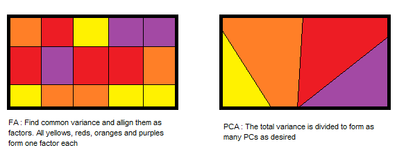
Source: This image is recreated from an image that I found in factor analysis notes. The image gives a full view of factor analysis.

Assumptions:

1. There are no outliers in data.
2. The sample size should be greater than the factor.
3. There should not be perfect multicollinearity.
4. There should not be homoscedasticity between the variables.

Types of Factor Analysis

• Exploratory Factor Analysis: It is the most popular factor analysis approach among social and management researchers. Its basic assumption is that any observed variable is directly associated with any factor.
• Confirmatory Factor Analysis (CFA): Its basic assumption is that each factor is associated with a particular set of observed variables. CFA confirms what is expected on the basis.

How does factor analysis work?

The primary objective of factor analysis is to reduce the number of observed variables and find unobservable variables. These unobserved variables help the market researcher to conclude the survey. This conversion of the observed variables to unobserved variables can be achieved in two steps:

• Factor Extraction: In this step, the number of factors and approach for extraction selected using variance partitioning methods such as principal components analysis and common factor analysis.
• Factor Rotation: In this step, rotation tries to convert factors into uncorrelated factors — the main goal of this step to improve the overall interpretability. There are lots of rotation methods that are available such as the Varimax rotation method, Quartimax rotation method, and Promax rotation method.

Terminology

What is a factor?

A factor is a latent variable that describes the association among the number of observed variables. The maximum number of factors is equal to a number of observed variables. Every factor explains a certain variance in observed variables. The factors with the lowest amount of variance were dropped. Factors are also known as latent variables or hidden variables or unobserved variables or Hypothetical variables.

What are the factor loadings?

The factor loading is a matrix that shows the relationship of each variable to the underlying factor. It shows the correlation coefficient for observed variables and factors. It shows the variance explained by the observed variables.

What is Eigenvalues?

Eigenvalues represent variance explained each factor from the total variance. It is also known as characteristic roots.

What are Communalities?

Commonalities are the sum of the squared loadings for each variable. It represents the common variance. It ranges from 0–1 and value close to 1 represents more variance.

What is Factor Rotation?

Rotation is a tool for better interpretation of factor analysis. Rotation can be orthogonal or oblique. It re-distributed the commonalities with a clear pattern of loadings.

Choosing the Number of Factors

Kaiser criterion is an analytical approach, which is based on the more significant proportion of variance explained by a factor that will be selected. The eigenvalue is a good criterion for determining the number of factors. Generally, an eigenvalue greater than 1 will be considered as the selection criteria for the feature.

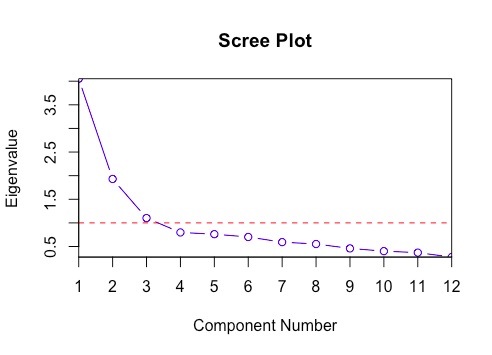
The graphical approach is based on the visual representation of factors’ eigenvalues also called scree plots. This scree plot helps us to determine the number of factors where the curve makes an elbow.

Factor Analysis Vs. Principle Component Analysis

• PCA components explain the maximum amount of variance while factor analysis explains the covariance in data.
• PCA components are fully orthogonal to each other whereas factor analysis does not require factors to be orthogonal.
• PCA component is a linear combination of the observed variable while in FA, the observed variables are linear combinations of the unobserved variable or factor.
• PCA components are uninterpretable. In FA, underlying factors are labelable and interpretable.
• PCA is a kind of dimensionality reduction method whereas factor analysis is the latent variable method.
• PCA is a type of factor analysis. PCA is observational whereas FA is a modeling technique.

Factor Analysis in Python using factor_analyzer package

Import Required Libraries

# Import required libraries
import pandas as pd
from sklearn.datasets import load_iris
from factor_analyzer import FactorAnalyzer
import matplotlib.pyplot as plt

Loading Data

Let’s perform factor analysis on BFI (dataset based on personality assessment project), which were collected using a 6 point response scale: 1 Very Inaccurate, 2 Moderately Inaccurate, 3 Slightly Inaccurate 4 Slightly Accurate, 5 Moderately Accurate, and 6 Very Accurate. You can also download this dataset from the following the link: https://vincentarelbundock.github.io/Rdatasets/datasets.html

df= pd.read_csv("bfi.csv")

Preprocess Data

df.columnsOutput:Index(['A1', 'A2', 'A3', 'A4', 'A5', 'C1', 'C2', 'C3', 'C4', 'C5', 'E1', 'E2','E3', 'E4', 'E5', 'N1', 'N2', 'N3', 'N4', 'N5', 'O1', 'O2', 'O3', 'O4','O5', 'gender', 'education', 'age'],dtype='object')# Dropping unnecessary columns
df.drop(['gender', 'education', 'age'],axis=1,inplace=True)# Dropping missing values rows
df.dropna(inplace=True)df.info()Output:<class 'pandas.core.frame.DataFrame'>
Int64Index: 2436 entries, 0 to 2799
Data columns (total 25 columns):
A1    2436 non-null float64
A2    2436 non-null float64
A3    2436 non-null float64
A4    2436 non-null float64
A5    2436 non-null float64
C1    2436 non-null float64
C2    2436 non-null float64
C3    2436 non-null float64
C4    2436 non-null float64
C5    2436 non-null float64
E1    2436 non-null float64
E2    2436 non-null float64
E3    2436 non-null float64
E4    2436 non-null float64
E5    2436 non-null float64
N1    2436 non-null float64
N2    2436 non-null float64
N3    2436 non-null float64
N4    2436 non-null float64
N5    2436 non-null float64
O1    2436 non-null float64
O2    2436 non-null int64
O3    2436 non-null float64
O4    2436 non-null float64
O5    2436 non-null float64
dtypes: float64(24), int64(1)
memory usage: 494.8 KBdf.head()Output:

Adequacy Test

Before you perform factor analysis, you need to evaluate the “factorability” of our dataset. Factorability means “can we found the factors in the dataset?”. There are two methods to check the factorability or sampling adequacy:

• Bartlett’s Test
• Kaiser-Meyer-Olkin Test

Bartlett’s test of sphericity checks whether or not the observed variables intercorrelate at all using the observed correlation matrix against the identity matrix. If the test found statistically insignificant, you should not employ a factor analysis.

from factor_analyzer.factor_analyzer import calculate_bartlett_sphericity
chi_square_value,p_value=calculate_bartlett_sphericity(df)
chi_square_value, p_valueOutput:(18146.065577234807, 0.0)

In Bartlett’s test, the p-value is 0. The test was statistically significant, indicating that the observed correlation matrix is not an identity matrix.

Kaiser-Meyer-Olkin (KMO) Test measures the suitability of data for factor analysis. It determines the adequacy for each observed variable and for the complete model. KMO estimates the proportion of variance among all the observed variables. Lower proportion id more suitable for factor analysis. KMO values range between 0 and 1. The value of KMO less than 0.6 is considered inadequate.

from factor_analyzer.factor_analyzer import calculate_kmo
kmo_all,kmo_model=calculate_kmo(df)kmo_modelOutput:0.8486452309468382

The overall KMO for our data is 0.84, which is excellent. This value indicates that you can proceed with your planned factor analysis.

Choosing the Number of Factors

For choosing the number of factors, you can use the Kaiser criterion and scree plot. Both are based on eigenvalues.

# Create factor analysis object and perform factor analysis
fa = FactorAnalyzer()
fa.analyze(df, 25, rotation=None)
# Check Eigenvalues
ev, v = fa.get_eigenvalues()
ev

Here, you can see only for 6-factors eigenvalues are greater than one. It means we need to choose only 6 factors (or unobserved variables).

# Create scree plot using matplotlib
plt.scatter(range(1,df.shape[1]+1),ev)
plt.plot(range(1,df.shape[1]+1),ev)
plt.title('Scree Plot')
plt.xlabel('Factors')
plt.ylabel('Eigenvalue')
plt.grid()
plt.show()

The scree plot method draws a straight line for each factor and its eigenvalues. Number eigenvalues greater than one considered as the number of factors.

Here, you can see only for 6-factors eigenvalues are greater than one. It means we need to choose only 6 factors (or unobserved variables).

Performing Factor Analysis

# Create factor analysis object and perform factor analysis
fa = FactorAnalyzer()
fa.analyze(df, 6, rotation="varimax")fa.loadings

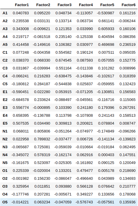
• Factor 1 has high factor loadings for E1,E2,E3,E4, and E5 (Extraversion)
• Factor 2 has high factor loadings for N1, N2, N3, N4, and N5 (Neuroticism)
• Factor 3 has high factor loadings for C1, C2, C3, C4, and C5 (Conscientiousness)
• Factor 4 has a high factor loadings for O1, O2, O3, O4, and O5 (Openness)
• Factor 5 has high factor loadings for A1, A2, A3, A4, and A5 (Agreeableness)
• Factor 6 has none of the high loadings for any variable and is not easily interpretable. It’s good if we take only five factors.

Let’s perform a factor analysis for 5 factors.

# Create factor analysis object and perform factor analysis using 5 factors
fa = FactorAnalyzer()
fa.analyze(df, 5, rotation="varimax")
fa.loadings

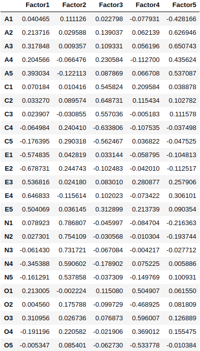
# Get variance of each factors
fa.get_factor_variance()

Total 42% cumulative Variance explained by the 5 factors.

Pros and Cons of Factor Analysis

Factor analysis explores large datasets and finds interlinked associations. It reduces the observed variables into a few unobserved variables or identifies the groups of inter-related variables, which help the market researchers to compress the market situations and find the hidden relationship among consumer taste, preference, and cultural influence. Also, It helps in improving the questionnaire for future surveys. Factors make for more natural data interpretation.

The results of the factor analysis are controversial. Its interpretations can be debatable because more than one interpretation can be made of the same data factors. After factor identification and naming of factors requires domain knowledge.

Conclusion

Congratulations, you have made it to the end of this tutorial!

In this tutorial, you have learned what factor analysis is. The different types of factor analysis, how does factor analysis work, basic factor analysis terminology, choosing the number of factors, comparison of principal component analysis and factor analysis, implementation in Python using Python FactorAnalyzer package, and pros and cons of factor analysis.

I look forward to hearing any feedback or questions. you can ask the question by leaving a comment and I will try my best to answer it.

Originally published at https://www.datacamp.com/community/tutorials/introduction-factor-analysis

Reach out to me on Linkedin: https://www.linkedin.com/in/avinash-navlani/