
Dimensionality Reduction using tSNE
tSNE stands for t-distributed Stochastic Neighbor Embedding. It is a dimensionality reduction technique and is extremely useful for visualizing datasets with high dimensions.
Dimensionality reduction is the way to reduce the number of features in a model along with preserving the important information that the data carries.
Data Visualization is extremely difficult in data with high dimensions, as the human eye can visualize up to three dimensions. tSNE reduces the higher dimensional data to 2D or 3D, which makes visualization easier.
tSNE is a non-linear, probabilistic technique. Dimensionality reduction algorithms like PCA (linear algorithm), fail to retain non-linear variance for the data (as it retains only the total variance for the data). tSNE, on the other hand, retains the local structure of the data. Since tSNE is a probabilistic technique, hence the results on the same data would slightly vary from each other. The probability distribution is modeled around the neighbors (closest points) of each data point. It is modeled as a Gaussian distribution in the high-dimensional space while the modeling in the 2D, i.e., lower-dimensional space is t-distribution. The algorithm tries to find a mapping onto the 2D space that minimizes the differences between these two distributions (the Kullback-Leibler divergence) for all points.
For the tSNE algorithm, two hyperparameters have considerable influence on the dimensionality reduction. The first one is n_iter, which is the number of iterations required for optimization. This should be at least 250. The other hyperparameter is perplexity, which is almost equal to the number of nearest neighbors that the algorithm must consider.
Working of tSNE
- The algorithm calculates the probability distribution of pairs of data points in high-dimension. The probability is higher for similar points and is lower for dissimilar points.
- It then calculates the probability of similarity of those points in the corresponding low-dimension.
- The algorithm then tries to minimize the difference between the distribution between the higher and the lower dimensional spaces. tSNE uses a gradient descent method to minimize the sum of Kullback-Leibler divergence of over all the data points.
Python Example
Dimensionality reduction using tSNE can be performed using Python’s sklearn library’s function sklearn.manifold.TSNE(). Let’s consider the following data:
| # creating the dataset from sklearn.datasets import load_digits d = load_digits() |
This is the MNIST data set that contains the digit data (i.e., the digits from 0 to 9). We can look at the dimensionality of this data, using:
| print(d.data.shape) |
This gives the output as (1797, 64). There are a total of 1797 data points. The dimensionality of this dataset is 64. Each data point is an 8×8 image of a digit, so there are 10 classes, i.e., the digits 0 to 9. We will reduce the dimensions of this data from 64 to a lower value.
First, let’s store the data and target variables in x and y, as:
| x, y = d.data, d.target |
The variable x is:
| print(x) |
Output:
| [[ 0. 0. 5. … 0. 0. 0.] [ 0. 0. 0. … 10. 0. 0.] [ 0. 0. 0. … 16. 9. 0.] … [ 0. 0. 1. … 6. 0. 0.] [ 0. 0. 2. … 12. 0. 0.] [ 0. 0. 10. … 12. 1. 0.]] |
And the variable y (which stores the actual digits) is:
| print(y) |
Output:
| [0 1 2 … 8 9 8] |
Both x and y are of length 1797. Now let’s perform dimensionality reduction with tSNE on this digits data, by reducing the data to 2-dimensions. This is done as:
| from sklearn.manifold import TSNE tsne = TSNE(n_components=2).fit_transform(x) |
The data has been reduced to 2-dimensions. The parameter n_components specifies the number of components in the reduced data. We can view the two-dimensional data as:
| print(tsne) |
Output:
| [[-62.74791 0.73374224] [ 18.917946 16.510155 ] [ 27.01022 -10.221348 ] … [ 19.968765 -0.17523506] [-12.308112 -11.3464575 ] [ 13.493948 -9.890771 ]] |
Now, let’s visualize the dimensionality reduction in a 2D plot. Let’s store this data in a DataFrame and then plot the points:
| import pandas as pd data = {‘x’:tsne[:,0], ‘y’:tsne[:,1], ‘dig’:y} df = pd.DataFrame(data) |
Let’s visualize the scatter plot:
| import matplotlib.pyplot as plt plt.scatter(df.x, df.y, c=df.dig, s=5) plt.show() |
Output:
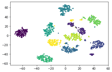
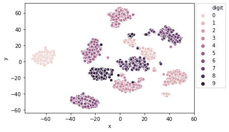
tSNE has classified the digits into their own clusters. The clusters for specific digits can be viewed more clearly as:
| import seaborn as sns sns.scatterplot(x=’x’, y=’y’, hue=’digit’, legend=’full’, data=df) plt.legend(bbox_to_anchor=(1.01, 1), borderaxespad=0) |
Output:
We can also change the hyperparameters to arrive at an optimal model.
Summary
In this article, we looked at Dimensionality Reduction using tSNE. In the next article, we will focus on ensemble techniques such as Bagging and Boosting.