MNIST with Julia

Today we write the “Hello World” of machine learning in Flux, training a simple neural net to classify hand-written digits from the MNIST database. As you’re here on Machine Learning Geek, I don’t believe you need any introduction to this, so let’s get right into the action.

Data Loading

First of all we load all the data using Flux‘s built-in functions:

using Flux
images = Flux.Data.MNIST.images();
labels = Flux.Data.MNIST.labels();

We can check out random images and labels:

using Random
x=rand(1:60000)
md"""
$(images[x])
# $(labels[x])"""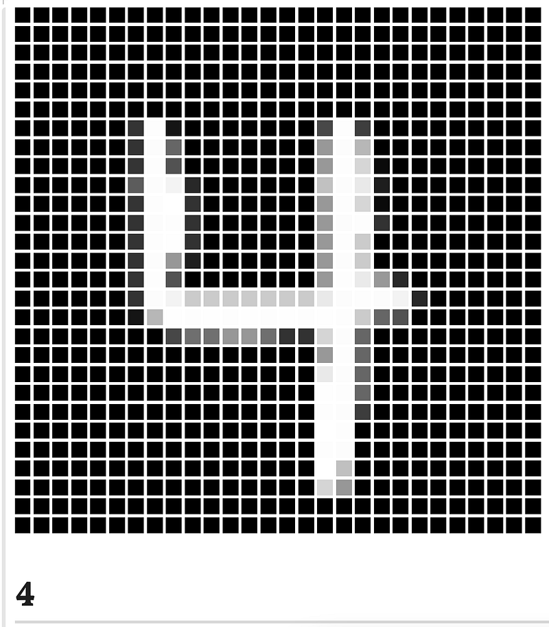

Preprocessing

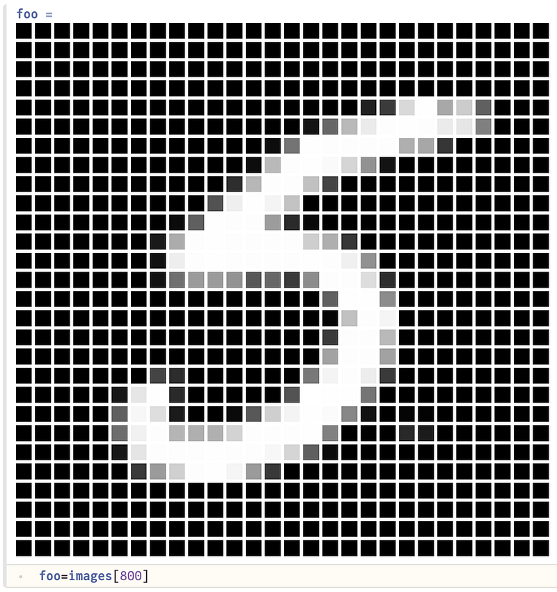
We’ll preprocess as usual. Lets pick an image:

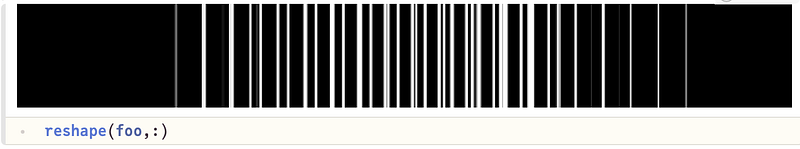
Now we’ll reshape it into a vector:

But currently, it’s a vector of fixed-point numbers, which won’t play well with our modeling:

So we’ll convert it into a floating-point vector:

Now we’ll apply these steps to all the images in one fell swoop, and then convert our image data into columns.

X=hcat(float.(reshape.(images,:))...)

Now we’ll use another function from Flux to one-hot encode our labels:

using Flux:onehotbatch
y = onehotbatch(labels, 0:9)

We’ll now define our model to consist of two fully connected layers, with a softmax at the end for easing inference:

m = Chain(
  Dense(28*28,40, relu),
  Dense(40, 10),
  softmax)

As you can see, our model takes in a 28\times 2828×28 array, runs it through the first layer to get a 40-dimensional vector, which the second layer then converts into a 10-dimenssional vector to be fed into the softmax activation function for inference. Now that we have the ingridents, lets put them together:

using Flux:crossentropy,onecold,throttle
loss(X, y) = crossentropy(m(X), y) 
opt = ADAM()

As is easy to figure out, we’re going to use log-loss as our loss function, and ADAM for gradient-descent. Finally, we’re going to define function to show us the loss after every epoch. This isn’t mandatory, but definitely enhances our quality of life.

progress = () -> @show(loss(X, y)) # callback to show loss

And now we train our model, and request it to report the loss every 10 seconds.

using Flux:@epochs
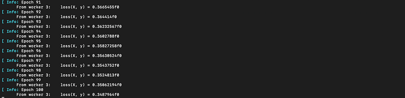
@epochs 100 Flux.train!(loss, params(m),[(X,y)], opt, cb = throttle(progress, 10))

As you probably remember from our last article on Flux, train! only trains for one epoch at a time, so we import and use the @epochs macro to train for 100 epochs. If you’re working in Pluto notebooks like me, do note that the progress the callback will print to your terminal:

…

Now that we’re done training, we ought to verify that our model is working well, so we check it on a random test image:

foobar=rand(1:10000)
	md"""
	$(Flux.Data.MNIST.images(:test)[foobar])
	# Prediction: $(onecold(m(hcat(float.(reshape.(Flux.Data.MNIST.images(:test), :))...)[:,foobar])) - 1)
	"""

Here’s how it looks in Pluto:

Bonus, if you want to check the accuracy of our training and test sets, the following terse code shall display it for you:

using Statistics:mean
	accuracy(X, y) = mean(onecold(m(X)) .== onecold(y))
	md"""
	# Training accuracy: $(accuracy(X, y))
	# Test accuracy: $(accuracy(hcat(float.(reshape.(Flux.Data.MNIST.images(:test), :))...), onehotbatch(Flux.Data.MNIST.labels(:test), 0:9)))"""

The above two code-blocks are simply applying our pre-processing steps to test data, and then displaying them in a pretty way.

Don’t worry if you don’t yet grok macros or Flux, this was just an appetizer, we’ll be hand-rolling a regression and an SVM model soon. As well as discussing Macros and Flux in more detail.

As usual, you can access the whole notebook at your leisure as well:

https://github.com/mathmetal/Misc/blob/master/MLG/MNIST.jl

References

1. https://fluxml.ai/Flux.jl/stable/data/onehot/
2. https://fluxml.ai/Flux.jl/stable/data/dataloader/