Backpropagation Neural Network using Python

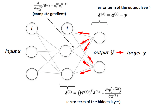
Backpropagation neural network is used to improve the accuracy of neural network and make them capable of self-learning. Backpropagation means “backward propagation of errors”. Here error is spread into the reverse direction in order to achieve better performance. 

Backpropagation is an algorithm for supervised learning of artificial neural networks that uses the gradient descent method to minimize the cost function. It searches for optimal weights that optimize the mean-squared distance between the predicted and actual labels.

In this tutorial, we are going to cover the following topics:

What is Backpropagation Neural Network(BPN)?

BPN was discovered by Rumelhart, Williams & Honton in 1986. The core concept of BPN is to backpropagate or spread the error from units of output layer to internal hidden layers in order to tune the weights to ensure lower error rates. It is considered a practice of fine-tuning the weights of neural networks in each iteration. Proper tuning of the weights will make a sure minimum loss and this will make a more robust, and generalizable trained neural network. 

How BPN works?

BPN learns in an iterative manner. In each iteration, it compares training examples with the actual target label. target label can be a class label or continuous value. The backpropagation algorithm works in the following steps:

• Initialize Network: BPN randomly initializes the weights. 
• Forward Propagate: After initialization, we will propagate into the forward direction. In this phase, we will compute the output and calculate the error from the target output.
• Back Propagate Error: For each observation, weights are modified in order to reduce the error in a technique called the delta rule or gradient descent. It modifies weights in a “backward” direction to all the hidden layers.

Implementation in Python

Import Libraries

Lets import the required modules and libraries such as numpy, pandas, scikit-learn, and matplotlib.

# Import Libraries
import numpy as np
import pandas as pd
from sklearn.datasets import load_iris
from sklearn.model_selection import train_test_split
import matplotlib.pyplot as plt

Load Dataset

Let’s first load the Iris dataset using load_iris() function of scikit-learn library and seprate them in features and target labels. This data set has three classes Iris-setosa, Iris-versicolor, and Iris-virginica.

# Load dataset
data = load_iris()

# Get features and target
X=data.data
y=data.target

Prepare Dataset

Create dummy variables for class labels using get_dummies() function

# Get dummy variable 
y = pd.get_dummies(y).values

y[:3]

Output:

array([[1, 0, 0],
       [1, 0, 0],
       [1, 0, 0]], dtype=uint8)

Split train and test set

To understand model performance, dividing the dataset into a training set and a test set is a good strategy.

Let’s split dataset by using function train_test_split(). you need to pass basically 3 parameters features, target, and test_set size. Additionally, you can use random_state in order to get the same kind of train and test set.

#Split data into train and test data
X_train, X_test, y_train, y_test = train_test_split(X, y, test_size=20, random_state=4)

Initialize Hyperparameters and Weights

Lets initialize the hyperparameters such as learning rate, iterations, input size, number of hidden layers, and number of output layers.

# Initialize variables
learning_rate = 0.1
iterations = 5000
N = y_train.size

# number of input features
input_size = 4

# number of hidden layers neurons
hidden_size = 2 

# number of neurons at the output layer
output_size = 3  

results = pd.DataFrame(columns=["mse", "accuracy"])

Lets initialize the weights for hidden and output layers with random values.

# Initialize weights
np.random.seed(10)

# initializing weight for the hidden layer
W1 = np.random.normal(scale=0.5, size=(input_size, hidden_size))   

# initializing weight for the output layer
W2 = np.random.normal(scale=0.5, size=(hidden_size , output_size)) 

Helper Functions

Lets create helper functions such as sigmoid, mean_square_error, and accuracy.

def sigmoid(x):
    return 1 / (1 + np.exp(-x))

def mean_squared_error(y_pred, y_true):
    return ((y_pred - y_true)**2).sum() / (2*y_pred.size)
    
def accuracy(y_pred, y_true):
    acc = y_pred.argmax(axis=1) == y_true.argmax(axis=1)
    return acc.mean()

Backpropagation Neural Network

In this phase, we will create backpropagation neural network in three steps feedforward propagation, error calculation and backpropagation phase. Here , we will create a for loop for given number of iterations that execute the three steps(feedforward propagation, error calculation and backpropagation phase) and update the weights in each iteration.

for itr in range(iterations):    
    
    # feedforward propagation
    # on hidden layer
    Z1 = np.dot(x_train, W1)
    A1 = sigmoid(Z1)

    # on output layer
    Z2 = np.dot(A1, W2)
    A2 = sigmoid(Z2)
    
    
    # Calculating error
    mse = mean_squared_error(A2, y_train)
    acc = accuracy(A2, y_train)
    results=results.append({"mse":mse, "accuracy":acc},ignore_index=True )
    
    # backpropagation
    E1 = A2 - y_train
    dW1 = E1 * A2 * (1 - A2)

    E2 = np.dot(dW1, W2.T)
    dW2 = E2 * A1 * (1 - A1)

    
    # weight updates
    W2_update = np.dot(A1.T, dW1) / N
    W1_update = np.dot(x_train.T, dW2) / N

    W2 = W2 - learning_rate * W2_update
    W1 = W1 - learning_rate * W1_update

Plot MSE and Accuracy

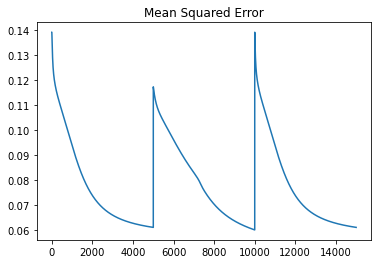
Lets plot mean squared error in each iteration using pandas plot() funciton.

results.mse.plot(title="Mean Squared Error")

Output:

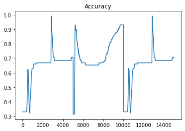
Lets plot accuracy in each iteration using pandas plot() funciton.

results.accuracy.plot(title="Accuracy")

Output:

Predict for Test Data and Evaluate the Performance

Lets make prediction for the test data and assess the performance of Backpropagation neural network.

# feedforward
Z1 = np.dot(x_test, W1)
A1 = sigmoid(Z1)

Z2 = np.dot(A1, W2)
A2 = sigmoid(Z2)

acc = accuracy(A2, y_test)
print("Accuracy: {}".format(acc))

Output:

Accuracy: 0.8

you can see in the above output, we are getting 80% accuracy on test dataset.

Pros and Cons

Backpropagation Neural Network is a simple and faster model compared to its earlier models. It is also a flexible and standard method. It does not need any prior knowledge for training. 

BPN performance depends upon the kind of input data is used. It is quite sensitive to noisy data. We need to use a matrix-based approach instead of a mini-batch. 

Conclusion

Congratulations, you have made it to the end of this tutorial!

Backpropagation neural network is a method to optimize neural networks by propagating the error or loss into a backward direction. It finds loss for each node and updates its weights accordingly in order to minimize the loss using gradient descent. 

In this tutorial, you have learned What is Backpropagation Neural Network, Backpropagation algorithm working, and Implementation from scratch in python. We have also discussed the pros and cons of the Backpropagation Neural Network.

References

• Basics of Deep Learning p.13 – Implementing the Backpropagation Algorithm with NumPy: https://www.sebastian-mantey.com/theory-blog/basics-of-deep-learning-p13-implementing-the-backpropagation-algorithm-with-numpy