Agglomerative Clustering
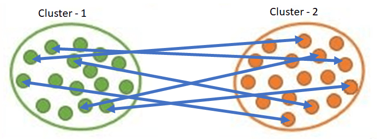
There are various different methods of Cluster Analysis, of which the Hierarchical Method is one of the most commonly used. In this method, the algorithm builds a hierarchy of clusters, where the data is organized in a hierarchical tree, as shown in the figure below:
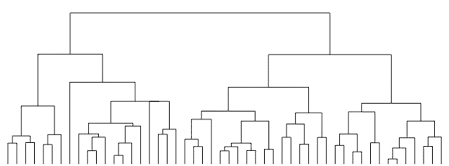
Hierarchical clustering has two approaches − the top-down approach (Divisive Approach) and the bottom-up approach (Agglomerative Approach). In this article, we will look at the Agglomerative Clustering approach.
Introduction
In Agglomerative Clustering, initially, each object/data is treated as a single entity or cluster. The algorithm then agglomerates pairs of data successively, i.e., it calculates the distance of each cluster with every other cluster. Two clusters with the shortest distance (i.e., those which are closest) merge and create a newly formed cluster which again participates in the same process. The algorithm keeps on merging the closer objects or clusters until the termination condition is met. This results in a tree-like representation of the data objects – dendrogram.
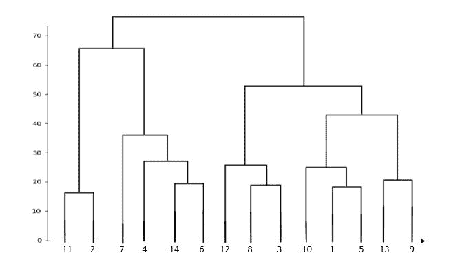
In the above dendrogram, we have 14 data points in separate clusters. In the dendrogram, the height at which two data points or clusters are agglomerated represents the distance between those two clusters in the data space.
Distance Metrics
The first step in agglomerative clustering is the calculation of distances between data points or clusters. Let’s look at some commonly used distance metrics:
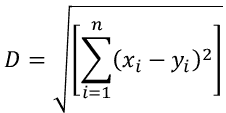
- Euclidean Distance:
It is the shortest distance between two points. In n-dimensional space:
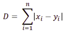
- Manhattan Distance:
Linkage
The linkage creation step in Agglomerative clustering is where the distance between clusters is calculated. So basically, a linkage is a measure of dissimilarity between the clusters. There are several methods of linkage creation. Some of them are:
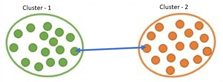
- Single Linkage
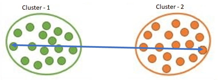
- Complete Linkage
- Average Linkage
In Single Linkage, the distance between the two clusters is the minimum distance between clusters’ data points.
In Complete Linkage, the distance between two clusters is the maximum distance between clusters’ data points.
In Average Linkage, the distance between clusters is the average distance between each data point in one cluster to every data point in the other cluster.
Example
Let’s take a look at an example of Agglomerative Clustering in Python. The function AgglomerativeClustering() is present in Python’s sklearn library.
Consider the following data:
| import pandas as pd data = [[200,500], [700,750], [250,450], [300,550], [600,300], [500,350], [700,850], [650,700], [900,700], [400,200]] df = pd.DataFrame(data, columns=[‘A’,’B’]) print(df) |
The DataFrame is:
| A B 0 200 500 1 700 750 2 250 450 3 300 550 4 600 300 5 500 350 6 700 850 7 650 700 8 900 700 9 400 200 |
Let’s view the dendrogram for this data. The python code to do so is:
| import scipy.cluster.hierarchy as sch dendrogram = sch.dendrogram(sch.linkage(df, method=’average’)) |
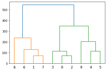
In this code, Average linkage is used. The dendrogram is:
Agglomerative Clustering function can be imported from the sklearn library of python. Looking at three colors in the above dendrogram, we can estimate that the optimal number of clusters for the given data = 3. Let’s create an Agglomerative clustering model using the given function by having parameters as:
| from sklearn.cluster import AgglomerativeClustering agg_model = AgglomerativeClustering(n_clusters=3, affinity=’euclidean’, linkage=’average’) agg_model.fit(df) |
The labels_ property of the model returns the cluster labels, as:
| cluster_label = agg_model.labels_ print(cluster_label) |
The labels for the above data are:
| [2 0 2 2 1 1 0 0 0 1] |
To visualize the clusters in the above data, we can plot a scatter plot as:
| # inserting the labels column in the original DataFrame df.insert(2, “Label”, cluster_label, True) # plotting the data import seaborn as sns sns.lmplot(data=df, x=’A’, y=’B’, hue=’Label’, fit_reg=False, legend=True, legend_out=True) |
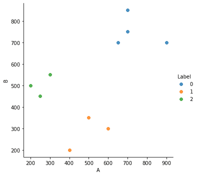
Visualization for the data and clusters is:
The above figure clearly shows the three clusters and the data points which are classified into those clusters.
Summary
In this article, we focused on Agglomerative Clustering. In the next article, we will look into DBSCAN Clustering.