Keras Tutorial for Beginners

In this tutorial, we will focus on Keras basics and learn neural network implementation using Keras. 

Keras is a widely used open-source deep-learning library for building neural network models. Keras offers a modular, easy to learn, easy to use, and faster prototype development framework. It is a higher-level wrapper of Tensorflow, CTNK, and Theano libraries. In the previous tutorial, we have seen  Introduction to Artificial Neural Network and  Multi-Layer Perceptron Neural Network using Python (using Scikit-learn). It’s time to jump on one of the best deep learning library Keras.

In this tutorial, we are going to cover the following topics:

What is Keras

Keras is a high-level deep learning python library for developing neural network models. Keras is a high-level API wrapper. It can run on top of the Tensorflow, CTNK, and Theano library. Keras is developed for the easy and fast development of neural network models.

Benefits and Limitations

Keras offers the following benefits:

• Keras is a Python library that is easy to learn and use framework.
• Faster development
• It can work on CPU and GPU.
• It can work with a variety of deep learning algorithms such as CNN, RNN, and LSTM.

Keras offers the following limitations:

• It depends upon lower-level libraries such as TensorFlow and Theano that can cause low-level errors.
• Only support NVIDIA GPU.
• Sometimes it is slower than its backend.

Keras Workflow

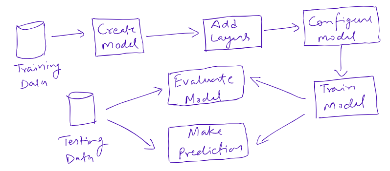
Keras Components

• Sequential Model: Keras provide an easy way to create multi-layer perception using the Sequential model. 
• Add Layer: add() function is used to add a layer to the neural network. We need to pass the type of layer we want to add to the sequential model.
• Dense Layer: It is a fully connected layer of neurons. It takes a number of nodes, activation function, and input_shape as the input parameters.
• Model Compilation: It is used to compile the model. It takes optimizer and loss function as the input parameters. The most popular optimization algorithms are Stochastic Gradient Descent (SGD), ADAM, and RMSprop. For the loss function, we can use Mean Squared Error (for regression problems), binary_crossentropy(for binary classification problem), or categorical_crossentropy(for multi-class classification).  
• Model Training: the fit() function used to train the model. It takes the following parameters as input: training data, validation data, and the number of epochs.
• Make Predictions: the predict() function is used to make predictions on new input data. 
• Model Evaluation: the evaluate() function is used to assess the model performance. it takes test features and labels as input.

Create Simple Neural Network

Import required libraries

import numpy as np
import pandas as pd

# Import scikit-learn modules
from sklearn import preprocessing
from sklearn.preprocessing import StandardScaler
from sklearn.model_selection import train_test_split

# Import keras modules
import keras
from keras.models import Sequential
from keras.layers import Dense

Load dataset

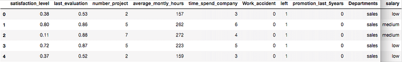
Let’s first load the required HR dataset using pandas’ read CSV function. You can download data from the following link: 

import numpy as np
import pandas as pd

# Load data
data=pd.read_csv('HR_comma_sep.csv')

data.head()

Output:

Preprocessing: Label Encoding and Feature Scaling

Lots of machine learning algorithms require numerical input data, so you need to represent categorical columns in a numerical column. In order to encode this data, you could map each value to a number. e.g. Salary column’s value can be represented as low:0, medium:1, and high:2. This process is known as label encoding. In sklearn, we can do this using LabelEncoder.

# Import LabelEncoder
from sklearn import preprocessing

# Creating labelEncoder
le = preprocessing.LabelEncoder()

# Converting string labels into numbers.
data['salary']=le.fit_transform(data['salary'])
data['Departments ']=le.fit_transform(data['Departments '])

# Convert dataframes into numpy array
X = X.values
y = y.values

# Scaling features
sc = StandardScaler()
X = sc.fit_transform(X)

Here, we imported the preprocessing module and created the Label Encoder object. Using this LabelEncoder object you fit and transform the “salary” and “Departments “ column into the numeric column.

Split the dataset

In order to assess the model performance, we need to divide the dataset into a training set and a test set. Let’s split dataset by using function train_test_split(). you need to pass basically 3 parameters features, target, and test_set size. 

# Split dataset into training set and test set
X_train, X_test, y_train, y_test = train_test_split(X, y, test_size=0.3, random_state=42)  # 70% training and 30% test

Create Neural Network Model

# Neural network
model = Sequential()

# Input layers
model.add(Dense(6, input_dim=9, activation='relu'))

# hidden layers
model.add(Dense(4, activation='relu'))

# Output Layer
model.add(Dense(1, activation='sigmoid'))

Compile and Train model

model.compile(loss='binary_crossentropy', 
              optimizer='adam', 
              metrics=['accuracy'])

model.fit(X_train, y_train, epochs=100, batch_size=64)

Epoch 1/100
188/188 [==============================] - 0s 1ms/step - loss: 0.6331 - accuracy: 0.6910
Epoch 2/100
188/188 [==============================] - 0s 900us/step - loss: 0.4697 - accuracy: 0.8192
Epoch 3/100
188/188 [==============================] - 0s 982us/step - loss: 0.3503 - accuracy: 0.8661
Epoch 4/100
188/188 [==============================] - 0s 814us/step - loss: 0.2707 - accuracy: 0.8983
Epoch 5/100
188/188 [==============================] - 0s 761us/step - loss: 0.2256 - accuracy: 0.9233
Epoch 6/100
188/188 [==============================] - 0s 651us/step - loss: 0.2011 - accuracy: 0.9370
Epoch 7/100
188/188 [==============================] - 0s 661us/step - loss: 0.1882 - accuracy: 0.9456
Epoch 8/100
188/188 [==============================] - 0s 766us/step - loss: 0.1808 - accuracy: 0.9487
Epoch 9/100
188/188 [==============================] - 0s 994us/step - loss: 0.1762 - accuracy: 0.9493
Epoch 10/100
188/188 [==============================] - 0s 923us/step - loss: 0.1731 - accuracy: 0.9498
Epoch 11/100
188/188 [==============================] - 0s 936us/step - loss: 0.1706 - accuracy: 0.9516
Epoch 12/100
188/188 [==============================] - 0s 821us/step - loss: 0.1690 - accuracy: 0.9519
Epoch 13/100
188/188 [==============================] - 0s 679us/step - loss: 0.1675 - accuracy: 0.9523
Epoch 14/100
188/188 [==============================] - 0s 844us/step - loss: 0.1662 - accuracy: 0.9524
Epoch 15/100
188/188 [==============================] - 0s 679us/step - loss: 0.1647 - accuracy: 0.9527
Epoch 16/100
188/188 [==============================] - 0s 969us/step - loss: 0.1640 - accuracy: 0.9524
Epoch 17/100
188/188 [==============================] - 0s 728us/step - loss: 0.1630 - accuracy: 0.9527
Epoch 18/100
188/188 [==============================] - 0s 546us/step - loss: 0.1624 - accuracy: 0.9533
Epoch 19/100
188/188 [==============================] - 0s 567us/step - loss: 0.1615 - accuracy: 0.9536
Epoch 20/100
188/188 [==============================] - 0s 530us/step - loss: 0.1610 - accuracy: 0.9544
Epoch 21/100
188/188 [==============================] - 0s 1ms/step - loss: 0.1604 - accuracy: 0.9535
Epoch 22/100
188/188 [==============================] - 0s 1ms/step - loss: 0.1597 - accuracy: 0.9544
Epoch 23/100
188/188 [==============================] - 0s 762us/step - loss: 0.1591 - accuracy: 0.9546
Epoch 24/100
188/188 [==============================] - 0s 776us/step - loss: 0.1584 - accuracy: 0.9546
Epoch 25/100
188/188 [==============================] - 0s 790us/step - loss: 0.1579 - accuracy: 0.9542
Epoch 26/100
188/188 [==============================] - 0s 568us/step - loss: 0.1575 - accuracy: 0.9552
Epoch 27/100
188/188 [==============================] - 0s 485us/step - loss: 0.1570 - accuracy: 0.9543
Epoch 28/100
188/188 [==============================] - 0s 445us/step - loss: 0.1563 - accuracy: 0.9557
Epoch 29/100
188/188 [==============================] - 0s 484us/step - loss: 0.1560 - accuracy: 0.9560
Epoch 30/100
188/188 [==============================] - 0s 487us/step - loss: 0.1552 - accuracy: 0.9561
Epoch 31/100
188/188 [==============================] - 0s 567us/step - loss: 0.1549 - accuracy: 0.9565
Epoch 32/100
188/188 [==============================] - 0s 1ms/step - loss: 0.1543 - accuracy: 0.9557
Epoch 33/100
188/188 [==============================] - 0s 779us/step - loss: 0.1541 - accuracy: 0.9561
Epoch 34/100
188/188 [==============================] - 0s 706us/step - loss: 0.1538 - accuracy: 0.9567
Epoch 35/100
188/188 [==============================] - 0s 682us/step - loss: 0.1532 - accuracy: 0.9568
Epoch 36/100
188/188 [==============================] - 0s 629us/step - loss: 0.1528 - accuracy: 0.9566
Epoch 37/100
188/188 [==============================] - 0s 607us/step - loss: 0.1523 - accuracy: 0.9572
Epoch 38/100
188/188 [==============================] - 0s 640us/step - loss: 0.1520 - accuracy: 0.9575
Epoch 39/100
188/188 [==============================] - 0s 561us/step - loss: 0.1516 - accuracy: 0.9575
Epoch 40/100
188/188 [==============================] - 0s 774us/step - loss: 0.1512 - accuracy: 0.9576
Epoch 41/100
188/188 [==============================] - 0s 897us/step - loss: 0.1512 - accuracy: 0.9575
Epoch 42/100
188/188 [==============================] - 0s 2ms/step - loss: 0.1506 - accuracy: 0.9574
Epoch 43/100
188/188 [==============================] - 0s 848us/step - loss: 0.1503 - accuracy: 0.9580
Epoch 44/100
188/188 [==============================] - 0s 1ms/step - loss: 0.1501 - accuracy: 0.9569
Epoch 45/100
188/188 [==============================] - 0s 1ms/step - loss: 0.1495 - accuracy: 0.9577
Epoch 46/100
188/188 [==============================] - 0s 1ms/step - loss: 0.1494 - accuracy: 0.9576
Epoch 47/100
188/188 [==============================] - 0s 1ms/step - loss: 0.1492 - accuracy: 0.9576
Epoch 48/100
188/188 [==============================] - 0s 1ms/step - loss: 0.1487 - accuracy: 0.9572
Epoch 49/100
188/188 [==============================] - 0s 958us/step - loss: 0.1484 - accuracy: 0.9580
Epoch 50/100
188/188 [==============================] - 0s 936us/step - loss: 0.1480 - accuracy: 0.9579
Epoch 51/100
188/188 [==============================] - 0s 1ms/step - loss: 0.1479 - accuracy: 0.9577
Epoch 52/100
188/188 [==============================] - 0s 1ms/step - loss: 0.1476 - accuracy: 0.9579
Epoch 53/100
188/188 [==============================] - 0s 1ms/step - loss: 0.1473 - accuracy: 0.9584
Epoch 54/100
188/188 [==============================] - 0s 1ms/step - loss: 0.1471 - accuracy: 0.9586
Epoch 55/100
188/188 [==============================] - 0s 757us/step - loss: 0.1470 - accuracy: 0.9581
Epoch 56/100
188/188 [==============================] - 0s 752us/step - loss: 0.1468 - accuracy: 0.9584
Epoch 57/100
188/188 [==============================] - 0s 875us/step - loss: 0.1464 - accuracy: 0.9587
Epoch 58/100
188/188 [==============================] - 0s 797us/step - loss: 0.1459 - accuracy: 0.9578
Epoch 59/100
188/188 [==============================] - 0s 774us/step - loss: 0.1461 - accuracy: 0.9578
Epoch 60/100
188/188 [==============================] - 0s 784us/step - loss: 0.1456 - accuracy: 0.9592
Epoch 61/100
188/188 [==============================] - 0s 955us/step - loss: 0.1453 - accuracy: 0.9582
Epoch 62/100
188/188 [==============================] - 0s 979us/step - loss: 0.1450 - accuracy: 0.9587
Epoch 63/100
188/188 [==============================] - 0s 1ms/step - loss: 0.1450 - accuracy: 0.9581
Epoch 64/100
188/188 [==============================] - 0s 818us/step - loss: 0.1449 - accuracy: 0.9585
Epoch 65/100
188/188 [==============================] - 0s 796us/step - loss: 0.1446 - accuracy: 0.9583
Epoch 66/100
188/188 [==============================] - 0s 799us/step - loss: 0.1444 - accuracy: 0.9589
Epoch 67/100
188/188 [==============================] - 0s 783us/step - loss: 0.1444 - accuracy: 0.9590
Epoch 68/100
188/188 [==============================] - 0s 795us/step - loss: 0.1441 - accuracy: 0.9592
Epoch 69/100
188/188 [==============================] - 0s 893us/step - loss: 0.1438 - accuracy: 0.9585
Epoch 70/100
188/188 [==============================] - 0s 799us/step - loss: 0.1437 - accuracy: 0.9588
Epoch 71/100
188/188 [==============================] - 0s 742us/step - loss: 0.1434 - accuracy: 0.9585
Epoch 72/100
188/188 [==============================] - 0s 843us/step - loss: 0.1433 - accuracy: 0.9590
Epoch 73/100
188/188 [==============================] - 0s 799us/step - loss: 0.1433 - accuracy: 0.9586
Epoch 74/100
188/188 [==============================] - 0s 811us/step - loss: 0.1429 - accuracy: 0.9584
Epoch 75/100
188/188 [==============================] - 0s 791us/step - loss: 0.1429 - accuracy: 0.9589
Epoch 76/100
188/188 [==============================] - 0s 765us/step - loss: 0.1426 - accuracy: 0.9587
Epoch 77/100
188/188 [==============================] - 0s 737us/step - loss: 0.1426 - accuracy: 0.9587
Epoch 78/100
188/188 [==============================] - 0s 827us/step - loss: 0.1423 - accuracy: 0.9585
Epoch 79/100
188/188 [==============================] - 0s 811us/step - loss: 0.1421 - accuracy: 0.9591
Epoch 80/100
188/188 [==============================] - 0s 845us/step - loss: 0.1419 - accuracy: 0.9588
Epoch 81/100
188/188 [==============================] - 0s 938us/step - loss: 0.1420 - accuracy: 0.9596
Epoch 82/100
188/188 [==============================] - 0s 747us/step - loss: 0.1418 - accuracy: 0.9594
Epoch 83/100
188/188 [==============================] - 0s 556us/step - loss: 0.1418 - accuracy: 0.9583
Epoch 84/100
188/188 [==============================] - 0s 479us/step - loss: 0.1418 - accuracy: 0.9592
Epoch 85/100
188/188 [==============================] - 0s 469us/step - loss: 0.1415 - accuracy: 0.9589
Epoch 86/100
188/188 [==============================] - 0s 702us/step - loss: 0.1415 - accuracy: 0.9590
Epoch 87/100
188/188 [==============================] - 0s 907us/step - loss: 0.1411 - accuracy: 0.9587
Epoch 88/100
188/188 [==============================] - 0s 1ms/step - loss: 0.1410 - accuracy: 0.9589
Epoch 89/100
188/188 [==============================] - 0s 951us/step - loss: 0.1413 - accuracy: 0.9580
Epoch 90/100
188/188 [==============================] - 0s 768us/step - loss: 0.1411 - accuracy: 0.9592
Epoch 91/100
188/188 [==============================] - 0s 967us/step - loss: 0.1406 - accuracy: 0.9587
Epoch 92/100
188/188 [==============================] - 0s 615us/step - loss: 0.1412 - accuracy: 0.9593
Epoch 93/100
188/188 [==============================] - 0s 1ms/step - loss: 0.1405 - accuracy: 0.9595
Epoch 94/100
188/188 [==============================] - 0s 965us/step - loss: 0.1404 - accuracy: 0.9592
Epoch 95/100
188/188 [==============================] - 0s 617us/step - loss: 0.1404 - accuracy: 0.9587
Epoch 96/100
188/188 [==============================] - 0s 615us/step - loss: 0.1403 - accuracy: 0.9586
Epoch 97/100
188/188 [==============================] - 0s 623us/step - loss: 0.1403 - accuracy: 0.9593
Epoch 98/100
188/188 [==============================] - 0s 605us/step - loss: 0.1401 - accuracy: 0.9591
Epoch 99/100
188/188 [==============================] - 0s 602us/step - loss: 0.1401 - accuracy: 0.9588
Epoch 100/100
188/188 [==============================] - 0s 714us/step - loss: 0.1401 - accuracy: 0.9591

Out[10]:

Evaluate model

score = model.evaluate(X_test, y_test,verbose=1)
print(score) #loss and accuracy

94/94 [==============================] - 0s 423us/step - loss: 0.1316 - accuracy: 0.9620
[0.1315860152244568, 0.9620000123977661]

Hyperparameter Tuning

In this section, we are covering the parameters that need to be hyper tune at the time of model building. We will learn the importance of each parameter in this section but we will see experimentation using all these parameters in upcoming articles.

Here is the list of parameters that need to tune during model training:

• The number of Dense layers and Number of nodes on each dense layer
• Optimization technique such as Stochastic Gradient Descent (SGD), ADAM, and RMSprop
• Type of activation function such as Mean Squared Error (for regression problems), binary_crossentropy(for binary classification problem), or categorical_crossentropy(for multi-class classification)
• Type of Network Topology: In the case of Convolutional Neural Network, We need to tune the filter size, pooling size, stride size, etc. 
• Loss function: Mean Square Error for regression, categorical cross-entropy for multi-class classification, binary cross-entropy for binary classification.
• Learning Rate: It is used to control the weight at the end of each epoch or how much the model can update its weight. 
• Momentum: It controls the influence of the previous weight update over the current weight update. It helps to prevent oscillations. A typical choice of momentum is between 0.5 to 0.9.
• Decay: It used to control the learning rate decay at the end of each epoch. 
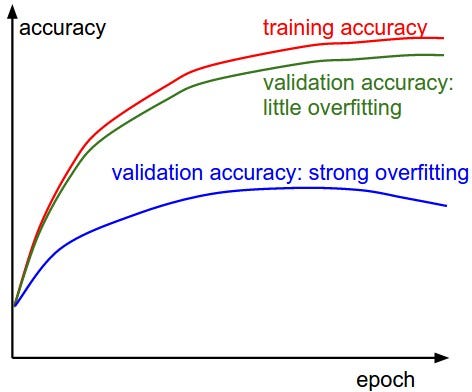
• Regularization for overcome overfitting.
• Dropout Rate: Dropout is a type of regularization technique that used to overcome overfitting in order to increase the model generalization power. 
• Batch Size: It is the number of training data samples used in each pass or iteration.
• The number of epochs: It defines the number of times the algorithm will scan through the entire training data.

Summary

Congratulations, you have made it to the end of this tutorial!

In this tutorial, we have discussed Keras library, workflow, components, benefits, and limitations. Also, we have built the classifier model for employee churn using the Neural Network classification model with Keras library in python.