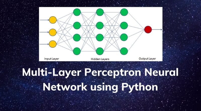
Multi-Layer Perceptron Neural Network using Python

In this tutorial, we will focus on the multi-layer perceptron, it’s working, and hands-on in python.

Multi-Layer Perceptron(MLP) is the simplest type of artificial neural network. It is a combination of multiple perceptron models. Perceptrons are inspired by the human brain and try to simulate its functionality to solve problems. In MLP, these perceptrons are highly interconnected and parallel in nature. This parallelization helpful in faster computation.

Perceptron

Perceptron was introduced by Frank Rosenblatt in 1950. It has the capability to learn complex things just like the human brain. Perceptron network consists of three units: Sensory Unit (Input Unit), Associator Unit (Hidden Unit), and Response Unit (Output Unit). 

How MLP works?

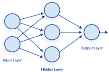
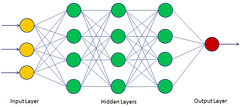
The Perceptron consists of an input layer and an output layer which are fully connected. MLPs have the same input and output layers but may have multiple hidden layers in between as mentioned in the previous section figure.

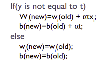
Multi-Layer Perceptron trains model in an iterative manner. In each iteration, partial derivatives of the loss function used to update the parameters. We can also use regularization of the loss function to prevent overfitting in the model.

Hands-on in Python

In this section, we will perform employee churn prediction using Multi-Layer Perceptron. Employee churn prediction helps us in designing better employee retention plans and improving employee satisfaction. For its exploratory data analysis you can refer to the following article on Predicting Employee Churn in Python:

Let’s start the model building hands-on in python.

Load dataset

Let’s first load the required HR dataset using pandas’ read CSV function. You can download data from the following link: 

import numpy as np
import pandas as pd

# Load data
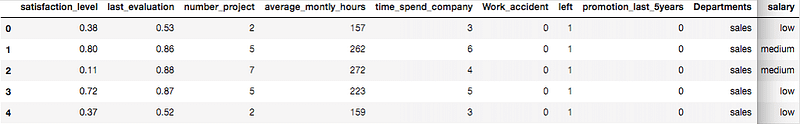
data=pd.read_csv('HR_comma_sep.csv')

data.head()

Output:

Preprocessing: Label Encoding

Lots of machine learning algorithms require numerical input data, so you need to represent categorical columns in a numerical column. In order to encode this data, you could map each value to a number. e.g. Salary column’s value can be represented as low:0, medium:1, and high:2. This process is known as label encoding. In sklearn, we can do this using LabelEncoder.

# Import LabelEncoder
from sklearn import preprocessing

# Creating labelEncoder
le = preprocessing.LabelEncoder()

# Converting string labels into numbers.
data['salary']=le.fit_transform(data['salary'])
data['Departments ']=le.fit_transform(data['Departments '])

Here, we imported the preprocessing module and created the Label Encoder object. Using this LabelEncoder object you fit and transform the “salary” and “Departments “ column into the numeric column.

Split the dataset

In order to assess the model performance, we need to divide the dataset into a training set and a test set. Let’s split dataset by using function train_test_split(). you need to pass basically 3 parameters features, target, and test_set size. 

# Spliting data into Feature and
X=data[['satisfaction_level', 'last_evaluation', 'number_project', 'average_montly_hours', 'time_spend_company', 'Work_accident', 'promotion_last_5years', 'Departments ', 'salary']]
y=data['left']

# Import train_test_split function
from sklearn.model_selection import train_test_split

# Split dataset into training set and test set
X_train, X_test, y_train, y_test = train_test_split(X, y, test_size=0.3, random_state=42)  # 70% training and 30% test

Build Classification Model

Let’s build an employee churn prediction model. Here, our objective is to predict churn using MLPClassifier.

First, import the MLPClassifier module and create MLP Classifier object using MLPClassifier() function. Then, fit your model on the train set using fit() and perform prediction on the test set using predict().

# Import MLPClassifer 
from sklearn.neural_network import MLPClassifier

# Create model object
clf = MLPClassifier(hidden_layer_sizes=(6,5),
                    random_state=5,
                    verbose=True,
                    learning_rate_init=0.01)

# Fit data onto the model
clf.fit(X_train,y_train)

Parameters:

• hidden_layer_sizes: it is a tuple where each element represents one layer and its value represents the number of neurons on each hidden layer.
• learning_rate_init: It used to controls the step-size in updating the weights. 
• activation: Activation function for the hidden layer. Examples, identity, logistic, tanh, and relu. by default, relu is used as an activation function.
• random_state: It defines the random number for weights and bias initialization. 
• verbose: It used to print progress messages to standard output.

Make Prediction and Evaluate the Model

In this section, we will make predictions on the test dataset and assess model accuracy based on available actual labels of the test dataset. 

# Make prediction on test dataset
ypred=clf.predict(X_test)

# Import accuracy score 
from sklearn.metrics import accuracy_score

# Calcuate accuracy
accuracy_score(y_test,ypred)

Output:
0.9386666666666666

Well, you got a classification rate of 93.8%, considered as good accuracy.

Summary

Congratulations, you have made it to the end of this tutorial!

In this tutorial, we have discussed perception, multilayer perception, it’s working, and MLP Classifier hands-on with python. we have built the classifier model for employee churn using Multi-Layer Perceptron Classification with the scikit-learn package.