Recurrent Neural Networks

Recurrent Neural Networks are special kinds of deep learning networks that were meant specially for dealing with sequence modeling problems. Whenever we have data in which the sequence of data matters like language translation, speech to text conversion, DNA sequence analysis, etc., we use RNN. The working logic of RNN states that the output of the current state not only depends on the current input but also on the previous state saved inside the cell, about the past inputs.

In this tutorial, we are going to cover the following topics:

Real-Life Applications of RNN

• Auto-sentence completion: You can see this while writing your emails on Gmail. Just after writing a few words, it automatically suggests a complete sentence.
• Text Summarization: Briefing a large text, preserving all the key information in a concise way.
• Language Translation: Since RNN can handle variable-length input data, it is quite ideal for language translation.
• Time Series forecasting: For predicting the price of stocks, weather forecasting, or sales of a product in the next quarter, RNN can solve the problem.

Benefits of RNN over feed-forward neural networks

• The usual feed-forward neural network assumes that the inputs are independent of each other but when it comes to sequential data, the order of input becomes important.
• RNN can handle variable-length input data, unlike other feed-forward networks.
• The feature which makes RNNs unique is that they have internal memory which makes them suitable for sequential data.
• The output of the current state not only depends on the current input but also on the previous state of the past inputs.
• In feed-forward networks, the flow of information is one-directional i.e., from input to output layer but RNN has the concept of a temporal loop. This loop helps RNN preserve information as memory.
• Weights are shared across time.

How does RNN work?

A regular deep learning network consists of the input layer, hidden layers, and an output layer. RNNs are also pretty much the same with slight modifications. Consider this diagram, showing the input, hidden layer, and output with a temporal loop.

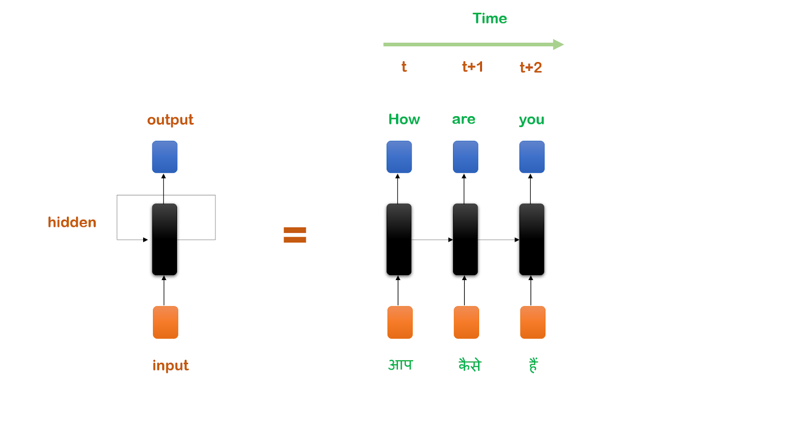
Suppose we are solving a language translation problem and we want to know the translation of a sentence. 

• A vector will be supplied as input (corresponding to the first word of the sentence) which will be passed into the hidden layer to finally produce the output.
• Now comes the interesting part, this information produced will be sent back into the network along with the vector for the next word in the sentence. Now the hidden layer will have two inputs which will produce a new output.
• This process is repeated until the last word of the sentence is reached, to finally translate the complete sentence.

Note: Machine translation is performed with the help of an encoder-decoder, we just used this example to get an idea of how RNN actually works.

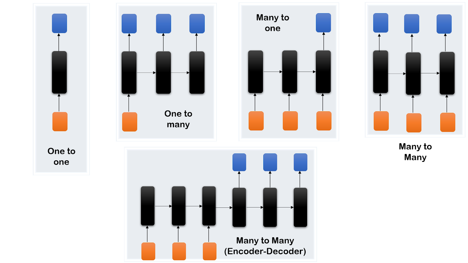
Types of RNN

• One to One:  For problems with only single input and a single output. 
• One to Many:  This is for vector to sequence problems. For example, using an image as an input to produce an image caption as text.
• Many to One:  A sequence of inputs is supplied to produce a single output, like in the case of sentiment analysis.
• Many to Many: This is used when RNN takes a sequence of input to produce another sequence as output. Example – Language translation, speech recognition. 

Stock Price prediction with RNN

We will be predicting the closing price of Netflix stocks with the help of RNN. For this, we will be using data from the year 2010 to 2022. 

Installing Packages

Using padas-datareader helps fetch data of various stocks from various sources. If you are using Google Colab  try using :

pip install --upgrade pandas-datareader

pip install pandas-datareader

Importing Libraries

import numpy as np
import pandas as pd
import pandas_datareader as pdr
import matplotlib.pyplot as plt
from datetime import datetime

Reading data

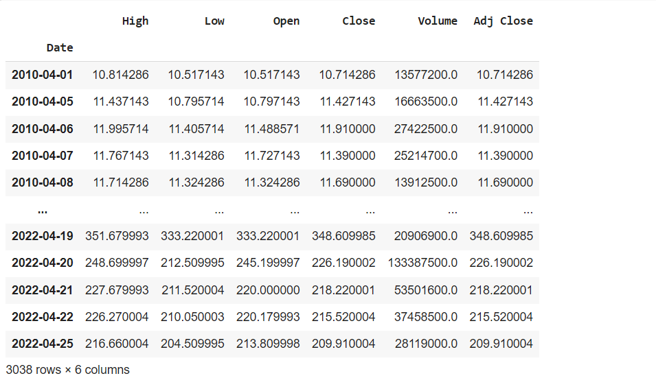
Pandas datareader provides a function get_data_yahoo to directly fetch the stock data of the specified stock from Yahoo Finance for the given duration. WE are extracting the Netflix stock price between the duration from 2010-04-01 to 2022-04-25.

df_netflix = pdr.get_data_yahoo('NFLX', start = '2010-04-01',end = '2022-04-25')
df_netflix

Visualizing data

Let us plot the Closing price of the stock for the past 12 years.

df = df_netflix['Close']
plt.figure(figsize = (15,4))
plt.plot(df)
plt.title("Closing Price")
plt.show()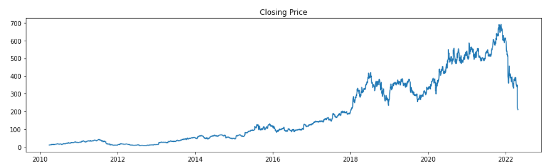

Dividing the dataset

Since this is time-series data, we cannot use the scikit-learn train_test_split() function because we need to preserve the order of prices. So, we will use, starting 80% of the values as a training dataset and the rest for testing. We also reshaped the datasets to make them compatible for the next step which is normalization. 

last_index = int(len(df) * 0.8)
train = df[:last_index].values.reshape(-1,1)
test = df[last_index:].values.reshape(-1,1)
train.shape, test.shape

((2430, 1), (608, 1))

Normalization

Normalization converts all the values in the range of 0 to 1. It improves convergence and hence reduces training time.

from sklearn.preprocessing import MinMaxScaler
 
scaler = MinMaxScaler()
train = scaler.fit_transform(train)
test = scaler.transform(test)
train[:10]

Splitting the dataset into X and Y

This function specifies how many previous values must be considered to find out the pattern, in order to predict a price. Accordingly, both, the training and testing datasets are split into X and Y.

def create_dataset(dataset, time_step=1):
  data_X, data_Y = [], []
  for i in range(len(dataset)-time_step-1):
    a = dataset[i:(i + time_step), 0]   
    data_X.append(a)
    data_Y.append(dataset[i + time_step, 0])
  return np.array(data_X), np.array(data_Y)

time_step = 100
X_train, y_train = create_dataset(train, 100)
X_test, y_test = create_dataset(test, 100)

Reshaping

To make the shape of the input compatible with the model we need to reshape it.

X_train = X_train.reshape(X_train.shape[0],X_train.shape[1], 1)
X_test = X_test.reshape(X_test.shape[0],X_test.shape[1], 1)

Building Model

For building the RNN model we stacked 3 recurrent layers using Keras SimpleRNN() function. Writing return_sequences = True ensures that the output is a 3D array containing outputs for all the time steps ready to be fed into the next recurrent layer (Not needed for the last layer because we only want the last output). For compiling the model adam optimizer is used and mean_squared_error as the loss function. At last, the summary of the model is shown.

from keras.models import Sequential
from keras.layers import SimpleRNN, Dense
 
model = Sequential([SimpleRNN(20, return_sequences = True, input_shape = [None,1]),
                    SimpleRNN(20, return_sequences = True),
                    SimpleRNN(20),
                    Dense(1)])
model.compile(loss = 'mean_squared_error', optimizer = 'adam')
model.summary()

Output:
Model: "sequential"
_________________________________________________________________
 Layer (type)                Output Shape              Param #   
=================================================================
 simple_rnn (SimpleRNN)      (None, None, 20)          440       
                                                                 
 simple_rnn_1 (SimpleRNN)    (None, None, 20)          820       
                                                                 
 simple_rnn_2 (SimpleRNN)    (None, 20)                820       
                                                                 
 dense (Dense)               (None, 1)                 21        
                                                                 
=================================================================
Total params: 2,101
Trainable params: 2,101
Non-trainable params: 0

Model training

For training purposes, we need to give training datasets and for testing, testing datasets along with respective labels and specify epochs (no. of iterations).

model.fit(X_train, y_train, validation_data = (X_test, y_test), epochs = 80)

Output:
Epoch 1/80
73/73 [==============================] - 4s 58ms/step - loss: 1.6642e-04 - val_loss: 0.0030
Epoch 2/80
73/73 [==============================] - 4s 57ms/step - loss: 1.6279e-04 - val_loss: 0.0020
Epoch 3/80
73/73 [==============================] - 4s 59ms/step - loss: 1.8406e-04 - val_loss: 0.0022
Epoch 4/80
73/73 [==============================] - 4s 59ms/step - loss: 1.6228e-04 - val_loss: 0.0020
Epoch 5/80
73/73 [==============================] - 4s 59ms/step - loss: 1.5072e-04 - val_loss: 0.0025
.
.
.
Epoch 75/80
73/73 [==============================] - 4s 58ms/step - loss: 1.5850e-04 - val_loss: 0.0018
Epoch 76/80
73/73 [==============================] - 4s 59ms/step - loss: 1.9614e-04 - val_loss: 0.0023
Epoch 77/80
73/73 [==============================] - 4s 59ms/step - loss: 1.5352e-04 - val_loss: 0.0017
Epoch 78/80
73/73 [==============================] - 4s 60ms/step - loss: 1.5618e-04 - val_loss: 0.0016
Epoch 79/80
73/73 [==============================] - 4s 58ms/step - loss: 1.8878e-04 - val_loss: 0.0017
Epoch 80/80
73/73 [==============================] - 4s 57ms/step - loss: 1.7536e-04 - val_loss: 0.0019
<keras.callbacks.History at 0x7fc3132469d0>

Prediction

After training the model is ready to make the predictions on the testing dataset. 

test_predict = model.predict(X_test)
test_predict[:10]

array([[1.0299232 ],
       [1.0298218 ],
       [1.0012373 ],
       [1.0180799 ],
       [1.0012494 ],
       [1.0095133 ],
       [0.97529024],
       [0.98867863],
       [1.0026649 ],
       [0.99097246]], dtype=float32)

Inversing Transformation

Since we normalized the data earlier and converted all the values in the range 0 to 1, now we should inverse the transformation to get actual values. 

test_predict=scaler.inverse_transform(test_predict)

Visualizing the predictions

Here we have plotted actual and predicted stock prices for the test dataset. We can see that the model is performing fine.

plt.figure(figsize = (15,4))
plt.plot(scaler.inverse_transform(y_test.reshape(-1,1)), color = 'r', label = 'actual')
plt.plot(test_predict, color = 'b',label = 'predicted')
plt.legend()
plt.show()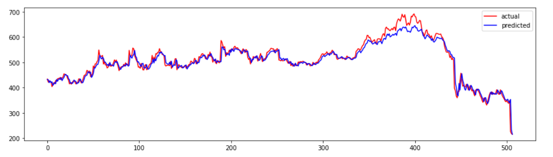

Evaluating model

For evaluation, we will be using root mean square values.

from sklearn.metrics import mean_squared_error
mean_squared_error(y_test,test_predict, squared = False)

Output:
507.0118272626747

Problems with RNN

• Vanishing Gradient: This happens when the gradient becomes very small and the weights hardly change, making the learning process very slow.
• Exploding Gradient: If the gradient happens to be a very large value, in this case, the weights would update drastically.
• Because of these two factors, it becomes very difficult to process long sequences of data if we are using relu or tanh as the activation function.
• Computation takes a lot of time because of the recurrent nature of the network.

Summary

In this tutorial, we have understood how a Recurrent Neural Network works. The feedback mechanism allows it to hold memory and this recurrent nature makes it ideal for sequence modeling problems. We have also implemented the RNN using python to predict the stock prices. In the upcoming session, we will try to focus on LSTM, GRU, and other deep learning topics. If you want to explore the Convolutional Neural Network (CNN) follow this article.