Understanding Convolutional Neural Network (CNN) using Python

April 19, 2022April 30, 2022 Tanisha Yadav

Learn the basics of the CNN model and perform image classification using Tensorflow and Keras.

Convolutional Neural Networks use filters on a given image at the pixel level and learn detailed patterns from it. Traditional Neural Network only captures the global patterns. CNN focuses on small patches in the image and develops a local level of understanding. In short, we can say convolution is the weighted sum of image pixel values.

In this tutorial, you are going to cover the following topics:

What CNN’s can do?

Cancer detection: CNNs have been proved quite accurate for the detection of cancer through CT scan images and mammograms.

Biometric Authentication: Whether the input is an image of a face, fingerprint, or iris, with the help of CNN biometric authentication can be performed with good accuracy.

Self-driving or autonomous cars: They are also used in self-driving cars for detecting obstacles and interpreting road signs which helps in better understanding of the environment.

Image captioning: It is the process of generating a brief description by automatically identifying the content of the image, supplied as input to the CNN model.
Handwritten character recognition: CNN models are capable of recognizing handwritten characters with good accuracy. Exp: Bank cheque processing, reading forms data, reading postal addresses, etc.

Why CNN?

Automatic Feature extraction therefore ideal for image classification problems.
In CNN all layers are not fully connected which reduces the amount of computation (which means fewer parameters to learn) unlike simple artificial neural networks.
CNN’s are invariant to the location of the object in the image and distortion in the scene.

How does CNN work?

Convolutional layer

This layer extracts important features from the input image such as horizontal lines, vertical lines, loops, etc. called feature maps.

To do so, we use a matrix of size N x N called filter or kernel.
We execute a convolution by sliding the filter over the input at every location, a matrix multiplication is performed and sums the result onto the feature map.
Because the size of the feature map is always smaller than the input, we have to do something to prevent our feature map from shrinking. This is where we use padding. A layer of zero-value pixels is added to surround the input with zeros so that our feature map will not shrink.

Convolution is followed by an activation function usually ReLU, whose output is the same as the input except it replaces all negative values with zero. This introduces non-linearity and speeds up training.

https://www.researchgate.net/publication/334974839_Graduation_Thesis_Implementing_and_Optimizing_Neural_Networks_using_Tiramisu

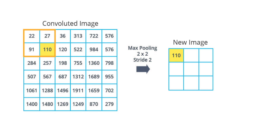
Pooling

A way to take large images and shrink them down while preserving the most important information in them
It consists of stepping a small window across an image and taking the maximum value from the window at each step – Max pooling. This window is swiped throughout the image.
The output will have the same number of images, but they will each have fewer pixels.
It reduces overfitting and makes the model tolerant of small distortion and variations.

Fully connected layers

This is where final classification takes place, but for this, we need the input to be in one dimension hence, first performing flattening. Then few fully connected layers are used with the last layer having exactly the same no. of neurons as the total no. of classes we have for classification.
It is also advised to add a dropout layer to avoid overfitting the training dataset by randomly dropping off a few neurons from the neural network during the training process.
Just before the final prediction, we use another activation function. For a binary classification CNN model, sigmoid and softmax functions are preferred and for multi-class classification, generally, softmax is used.

CIFAR-10 Dataset Image Classification with CNN

Now let’s see the python implementation of CNN with an example. Here we will be performing image classification with the help of CNN.

Dataset: CIFAR-10

There is a total of 60,000 images of 10 different classes naming Airplane, Automobile, Bird, Cat, Dog, Frog, Horse, Ship, Truck. All the images are of size 32×32. There are in total 50,000 train images and 10,000 test images.

Loading Dataset

Let’s first load the required CIFR-10 dataset from TensorFlow. You can also download data from the following link:

import numpy as np
import matplotlib.pyplot as plt
import tensorflow as tf 
 
cifar10 = tf.keras.datasets.cifar10
(X_train, y_train), (X_test, y_test) = cifar10.load_data()

print(X_train.shape, X_test.shape, y_train.shape, y_test.shape)

Output:
Downloading data from https://www.cs.toronto.edu/~kriz/cifar-10-python.tar.gz
170500096/170498071 [==============================] - 11s 0us/step
170508288/170498071 [==============================] - 11s 0us/step
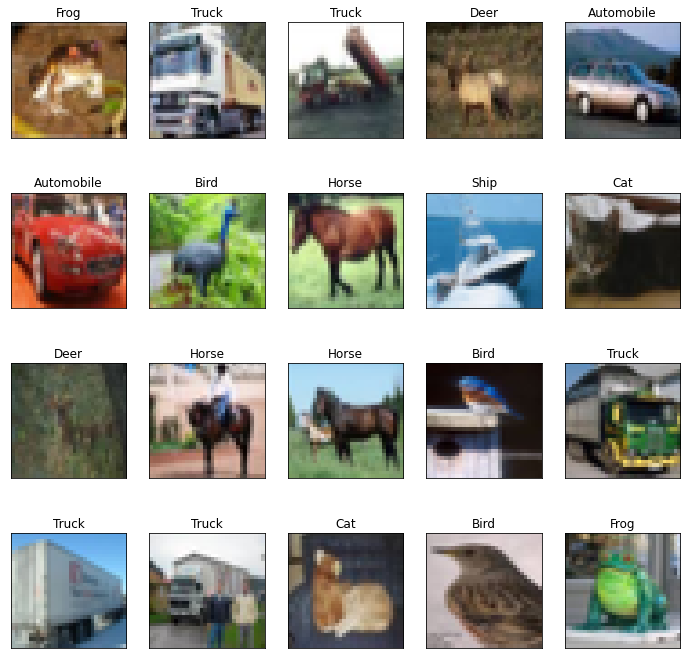
(50000, 32, 32, 3) (10000, 32, 32, 3) (50000, 1) (10000, 1)

View Dataset

labels = ['Airplane', 'Automobile', 'Bird', 'Cat', 'Deer', 'Dog', 'Frog', 'Horse', 'Ship', 'Truck']

fig, axes = plt.subplots(ncols = 5, nrows = 4, figsize = (12, 12))
 
index = 0 
for i in range(4):
  for j in range(5):
    axes[i,j].set_title(labels[y_train[index][0]])
    axes[i,j].imshow(X_train[index])
    axes[i,j].get_xaxis().set_visible(False)
    axes[i,j].get_yaxis().set_visible(False)
    index += 1

Output:

Normalization

X_train  = X_train/255.0
X_test  = X_test/255.0

One Hot Encoding

from tensorflow.keras.utils import to_categorical
 
y_train = tf.keras.utils.to_categorical(y_train, 10)
y_test = tf.keras.utils.to_categorical(y_test, 10)
y_train

Output:
array([[0., 0., 0., ..., 0., 0., 0.],
       [0., 0., 0., ..., 0., 0., 1.],
       [0., 0., 0., ..., 0., 0., 1.],
       ...,
       [0., 0., 0., ..., 0., 0., 1.],
       [0., 1., 0., ..., 0., 0., 0.],
 [0., 1., 0., ..., 0., 0., 0.]], dtype=float32)

Model Building

from keras.models import Sequential
from keras.layers import Conv2D, MaxPool2D, Flatten, Dense, Dropout, BatchNormalization
 
 
model = Sequential()
 
# Convolutional Layer
model.add(Conv2D(filters = 32, 
                 kernel_size = (3,3), 
                 input_shape = (32, 32, 3 ),
                 activation = 'relu',
                 padding='same'))
model.add(BatchNormalization())
model.add(Conv2D(filters=32, kernel_size=(3, 3), activation='relu', padding='same'))
model.add(BatchNormalization())
 
# Pooling layer
model.add(MaxPool2D( pool_size = (2,2)))
 
# Dropout Layer
model.add(Dropout(0.25))
 
 
model.add(Conv2D(filters=64, kernel_size=(3, 3), activation='relu', padding='same'))
model.add(BatchNormalization())
model.add(Conv2D(filters=64, kernel_size=(3, 3), activation='relu', padding='same'))
model.add(BatchNormalization())
 
model.add(MaxPool2D(pool_size=(2, 2)))
model.add(Dropout(0.25))
 
 
model.add(Conv2D(filters=128, kernel_size=(3, 3), activation='relu', padding='same'))
model.add(BatchNormalization())
model.add(Conv2D(filters=128, kernel_size=(3, 3), activation='relu', padding='same'))
model.add(BatchNormalization())
 
model.add(MaxPool2D(pool_size=(2, 2)))
model.add(Dropout(0.25))
 
# Flattening 
model.add(Flatten())
 
# Fully connected layers
model.add(Dense(128, activation = 'relu'))
model.add(Dropout(0.25))
model.add(Dense(10, activation = 'softmax'))

Compiling and training model

# compilation
model.compile(loss = 'categorical_crossentropy', optimizer = 'adam', 
metrics = 'accuracy')

# model training
model.fit(X_train, y_train, epochs=12)

Output:
Epoch 1/12
1563/1563 [==============================] - 43s 21ms/step - loss: 1.5208 - accuracy: 0.4551
Epoch 2/12
1563/1563 [==============================] - 28s 18ms/step - loss: 1.0673 - accuracy: 0.6272
Epoch 3/12
1563/1563 [==============================] - 33s 21ms/step - loss: 0.8979 - accuracy: 0.6908
Epoch 4/12
1563/1563 [==============================] - 33s 21ms/step - loss: 0.7959 - accuracy: 0.7270
Epoch 5/12
1563/1563 [==============================] - 32s 20ms/step - loss: 0.7143 - accuracy: 0.7558
Epoch 6/12
1563/1563 [==============================] - 32s 20ms/step - loss: 0.6541 - accuracy: 0.7752
Epoch 7/12
1563/1563 [==============================] - 32s 20ms/step - loss: 0.6077 - accuracy: 0.7933
Epoch 8/12
1563/1563 [==============================] - 32s 20ms/step - loss: 0.5655 - accuracy: 0.8072
Epoch 9/12
1563/1563 [==============================] - 32s 20ms/step - loss: 0.5324 - accuracy: 0.8197
Epoch 10/12
1563/1563 [==============================] - 31s 20ms/step - loss: 0.4913 - accuracy: 0.8322
Epoch 11/12
1563/1563 [==============================] - 32s 20ms/step - loss: 0.4754 - accuracy: 0.8385
Epoch 12/12
1563/1563 [==============================] - 32s 20ms/step - loss: 0.4413 - accuracy: 0.8491

Model Evaluation

prediction = model.evaluate(X_test, y_test)
print(f'Test Accuracy : {prediction[1] * 100:.2f}%')

Output:
313/313 [==============================] - 3s 9ms/step - loss: 0.5228 - accuracy: 0.8300
Test Accuracy : 83.00%

Pros

Automatic feature extraction without any human intervention.
Very High accuracy in image recognition problems.
Weight sharing – reducing the number of weights in a network that must be trained
It makes feature search insensitive to feature location in the image.

Cons

They are computationally expensive as the size of training images increases, and so is the number of computations.
CNN’s are slow to train if you don’t have GPU (for complex tasks).
Requires a lot of training data.
CNN’s cannot handle scaling or rotation of images automatically (without data augmentation).
CNN’s are incapable of effectively interpreting temporal information.

Tip

CNN by itself cannot take care of scaling or rotation of the image. So, therefore, you need to have scaled and rotated samples in the training dataset. In case you don’t have them in your dataset use data augmentation methods to generate new rotated/ scaled samples from the existing training samples.

Summary

In this tutorial, we have understood the fundamental concept of a Convolutional Neural Network. We have also gone through the detailed explanation of CNN components such as a convolutional layer, pooling layer, and fully connected layer. Finally, we implemented the CNN model for the CIFAR-10 dataset using the Keras library. If you are more interested in such articles please join the page on LinkedIn.

You can also prepare deep learning questions for the interview from the following article.