Solving Transportation Problem using Linear Programming in Python
Learn how to use Python PuLP to solve transportation problems using Linear Programming.
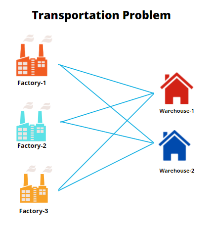
In this tutorial, we will broaden the horizon of linear programming problems. We will discuss the Transportation problem. It offers various applications involving the optimal transportation of goods. The transportation model is basically a minimization model.
The transportation problem is a type of Linear Programming problem. In this type of problem, the main objective is to transport goods from source warehouses to various destination locations at minimum cost. In order to solve such problems, we should have demand quantities, supply quantities, and the cost of shipping from source and destination. There are m sources or origin and n destinations, each represented by a node. The edges represent the routes linking the sources and the destinations.
In this tutorial, we are going to cover the following topics:
Transportation Problem
The transportation models deal with a special type of linear programming problem in which the objective is to minimize the cost. Here, we have a homogeneous commodity that needs to be transferred from various origins or factories to different destinations or warehouses.
Types of Transportation problems
- Balanced Transportation Problem: In such type of problem, total supplies and demands are equal.
- Unbalanced Transportation Problem: In such type of problem, total supplies and demands are not equal.
Methods for Solving Transportation Problem:
- NorthWest Corner Method
- Least Cost Method
- Vogel’s Approximation Method (VAM)
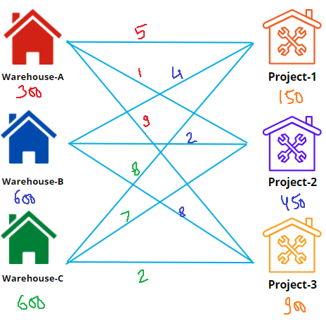
Let’s see one example below. A company contacted the three warehouses to provide the raw material for their 3 projects.
| Warehouse | Supply Capacity |
| A | 300 |
| B | 600 |
| C | 600 |
| Project | Demand Capacity |
| 1 | 150 |
| 2 | 450 |
| 3 | 900 |
| From | Project-1 | Project-2 | Project-3 |
| Warehouse-A | 5 | 1 | 9 |
| Warehouse-B | 4 | 2 | 8 |
| Warehouse-c | 8 | 7 | 2 |
This constitutes the information needed to solve the problem. The next step is to organize the information into a solvable transportation problem.
Formulate Problem
Let’s first formulate the problem. first, we define the warehouse and its supplies, the project and its demands, and the cost matrix.
# Creates a list of all the supply nodes
warehouses = ["A", "B", "C"]

# Creates a dictionary for the number of units of supply for each supply node
supply = {"A": 300, "B": 600, "C":600}

# Creates a list of all demand nodes
projects = ["1", "2", "3"]

# Creates a dictionary for the number of units of demand for each demand node
demand = {
    "1": 150,
    "2": 450,
    "3": 900,
}

# Creates a list of costs of each transportation path
costs = [  # Projects
    [5,1,9],  # A   warehouses
    [4,2,8],  # B
    [8,7,2]   # C
]

# The cost data is made into a dictionary
costs = makeDict([warehouses, projects], costs, 0)
Initialize LP Model
In this step, we will import all the classes and functions of pulp module and create a Minimization LP problem using LpProblem class.
# Import PuLP modeler functions
from pulp import *

# Creates the 'prob' variable to contain the problem data
prob = LpProblem("Material Supply Problem", LpMinimize)
Define Decision Variable
In this step, we will define the decision variables. In our problem, we have various Route variables. Let’s create them using LpVariable.dicts() class. LpVariable.dicts() used with Python’s list comprehension. LpVariable.dicts() will take the following four values:
- First, prefix name of what this variable represents.
- Second is the list of all the variables.
- Third is the lower bound on this variable.
- Fourth variable is the upper bound.
- Fourth is essentially the type of data (discrete or continuous). The options for the fourth parameter are
LpContinuousorLpInteger.
Let’s first create a list route for the route between warehouse and project site and create the decision variables using LpVariable.dicts() the method.
# Creates a list of tuples containing all the possible routes for transport
Routes = [(w, b) for w in warehouses for b in projects]

# A dictionary called 'Vars' is created to contain the referenced variables(the routes)
vars = LpVariable.dicts("Route", (warehouses, projects), 0, None, LpInteger)
Define Objective Function
In this step, we will define the minimum objective function by adding it to the LpProblem object. lpSum(vector)is used here to define multiple linear expressions. It also used list comprehension to add multiple variables.
# The minimum objective function is added to 'prob' first
prob += (
    lpSum([vars[w][b] * costs[w][b] for (w, b) in Routes]),
    "Sum_of_Transporting_Costs",
)
In this code, we have summed up the two variables(full-time and part-time) list values in an additive fashion.
Define the Constraints
Here, we are adding two types of constraints: supply maximum constraints and demand minimum constraints. We have added the 4 constraints defined in the problem by adding them to the LpProblem object.
# The supply maximum constraints are added to prob for each supply node (warehouses)
for w in warehouses:
    prob += (
        lpSum([vars[w][b] for b in projects]) <= supply[w],
        "Sum_of_Products_out_of_warehouses_%s" % w,
    )

# The demand minimum constraints are added to prob for each demand node (project)
for b in projects:
    prob += (
        lpSum([vars[w][b] for w in warehouses]) >= demand[b],
        "Sum_of_Products_into_projects%s" % b,
    )
Solve Model
In this step, we will solve the LP problem by calling solve() method. We can print the final value by using the following for loop.
# The problem is solved using PuLP's choice of Solver
prob.solve()

# Print the variables optimized value
for v in prob.variables():
    print(v.name, "=", v.varValue)

# The optimised objective function value is printed to the screen
print("Value of Objective Function = ", value(prob.objective))
Output: Route_A_1 = 0.0 Route_A_2 = 300.0 Route_A_3 = 0.0 Route_B_1 = 150.0 Route_B_2 = 150.0 Route_B_3 = 300.0 Route_C_1 = 0.0 Route_C_2 = 0.0 Route_C_3 = 600.0 Value of Objective Function = 4800.0
From the above results, we can infer that Warehouse-A supplies the 300 units to Project -2. Warehouse-B supplies 150, 150, and 300 to respective project sites. And finally, Warehouse-C supplies 600 units to Project-3.
Summary
In this article, we have learned about Transportation problems, Problem Formulation, and implementation using the python PuLp library. We have solved the transportation problem using a Linear programming problem in Python. Of course, this is just a simple case study, we can add more constraints to it and make it more complicated. In upcoming articles, we will write more on different optimization problems such as transshipment problem, assignment problem, balanced diet problem. You can revise the basics of mathematical concepts in this article and learn about Linear Programming in this article.