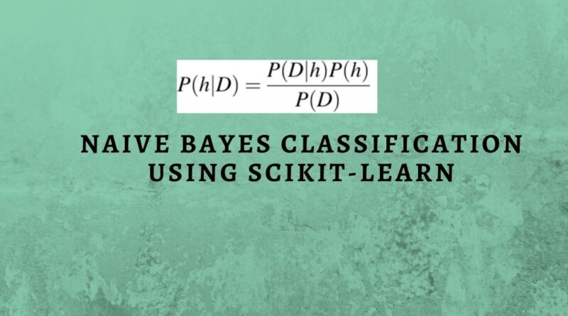
Naive Bayes Classification using Scikit-learn

March 19, 2021March 6, 2021 Avinash Navlani

Learn how to build and evaluate a Naive Bayes Classifier using Python’s Scikit-learn package.

Suppose you are a product manager, you want to classify customer reviews in positive and negative classes. Or As a loan manager, you want to identify which loan applicants are safe or risky? As a healthcare analyst, you want to predict which patients can suffer from diabetes disease. All the examples have the same kind of problem to classify reviews, loan applicants, and patients.

Naive Bayes is the most straightforward and fast classification algorithm, which is suitable for a large chunk of data. Naive Bayes classifier is successfully used in various applications such as spam filtering, text classification, sentiment analysis, and recommender systems. It uses Bayes theorem of probability for prediction of unknown class.

In this tutorial, you are going to learn about all of the following:

Classification Workflow
What is the Naive Bayes classifier?
How Naive Bayes classifier works?
Classifier building in Scikit-learn
Zero Probability Problem
It’s advantages and disadvantages

For more such tutorials, projects, and courses visit DataCamp:

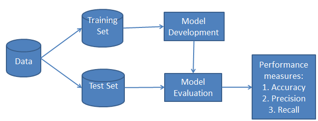
Classification Workflow

Whenever you perform classification, the first step is to understand the problem and identify potential features and labels. Features are those characteristics or attributes which affect the results of the label. For example, in the case of a loan distribution, the bank manager’s identify customer’s occupation, income, age, location, previous loan history, transaction history, and credit score. These characteristics are known as features that help the model classify customers.

The classification has two phases, a learning phase, and the evaluation phase. In the learning phase, the classifier trains its model on a given dataset, and in the evaluation phase, it tests the classifier performance. Performance is evaluated on the basis of various parameters such as accuracy, error, precision, and recall.

What is the Naive Bayes Classifier?

Naive Bayes is a statistical classification technique based on Bayes Theorem. It is one of the simplest supervised learning algorithms. Naive Bayes classifier is a fast, accurate, and reliable algorithm. Naive Bayes classifiers have high accuracy and speed on large datasets.

Naive Bayes classifier assumes that the effect of a particular feature in a class is independent of other features. For example, a loan applicant is desirable or not depending on his/her income, previous loan and transaction history, age, and location. Even if these features are interdependent, these features are still considered independently. This assumption simplifies computation, and that’s why it is considered as naive. This assumption is called class conditional independence.

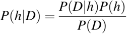
P(h): the probability of hypothesis h being true (regardless of the data). This is known as the prior probability of h.
P(D): the probability of the data (regardless of the hypothesis). This is known as the prior probability.
P(h|D): the probability of hypothesis h given the data D. This is known as posterior probability.
P(D|h): the probability of data d given that the hypothesis h was true. This is known as the posterior probability.

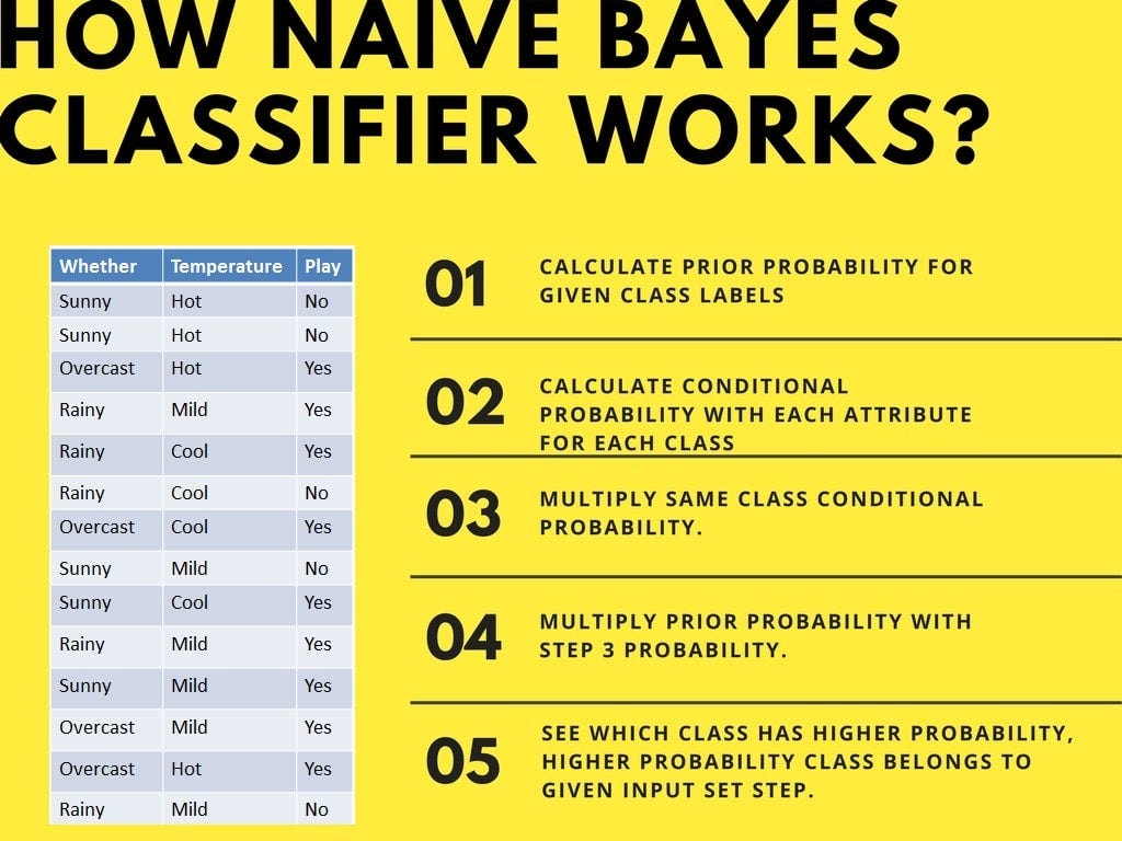
How Naive Bayes classifier works?

Let’s understand the working of Naive Bayes through an example. Given an example of weather conditions and playing sports. You need to calculate the probability of playing sports. Now, you need to classify whether players will play or not, based on the weather condition.

First Approach (In the case of a single feature)

Naive Bayes classifier calculates the probability of an event in the following steps:

Step 1: Calculate the prior probability for given class labels
Step 2: Find Likelihood probability with each attribute for each class
Step 3: Put these values in Bayes Formula and calculate posterior probability.
Step 4: See which class has a higher probability, given the input belongs to the higher probability class.

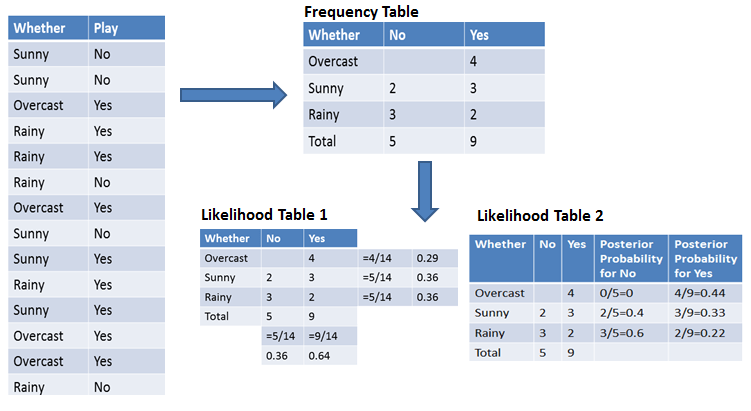
For simplifying prior and posterior probability calculation you can use the two tables frequency and likelihood tables. Both of these tables will help you to calculate the prior and posterior probability. The Frequency table contains the occurrence of labels for all features. There are two likelihood tables. Likelihood Table 1 is showing prior probabilities of labels and Likelihood Table 2 is showing the posterior probability.

Now suppose you want to calculate the probability of playing when the weather is overcast.

Probability of playing:

P(Yes | Overcast) = P(Overcast | Yes) P(Yes) / P (Overcast) …………………(1)

Calculate Prior Probabilities:
P(Overcast) = 4/14 = 0.29
P(Yes)= 9/14 = 0.64
Calculate Posterior Probabilities:
P(Overcast |Yes) = 4/9 = 0.44
Put Prior and Posterior probabilities in equation (1)
P (Yes | Overcast) = 0.44 * 0.64 / 0.29 = 0.98(Higher)

Similarly, you can calculate the probability of not playing:

Probability of not playing:

P(No | Overcast) = P(Overcast | No) P(No) / P (Overcast) …………………(2)

Calculate Prior Probabilities:
P(Overcast) = 4/14 = 0.29
P(No)= 5/14 = 0.36
Calculate Posterior Probabilities:
P(Overcast |No) = 0/9 = 0
Put Prior and Posterior probabilities in equation (2)
P (No | Overcast) = 0 * 0.36 / 0.29 = 0

The probability of a ‘Yes’ class is higher. So you can determine here if the weather is overcast than players will play the sport.

Second Approach (In case of multiple features)

Now suppose you want to calculate the probability of playing when the weather is overcast, and the temperature is mild.

Probability of playing:

P(Play= Yes | Weather=Overcast, Temp=Mild) = P(Weather=Overcast, Temp=Mild | Play= Yes)P(Play=Yes) ……….(1)

P(Weather=Overcast, Temp=Mild | Play= Yes)= P(Overcast |Yes) P(Mild |Yes) ………..(2)

Calculate Prior Probabilities: P(Yes)= 9/14 = 0.64
Calculate Posterior Probabilities: P(Overcast |Yes) = 4/9 = 0.44 P(Mild |Yes) = 4/9 = 0.44
Put Posterior probabilities in equation (2) P(Weather=Overcast, Temp=Mild | Play= Yes) = 0.44 * 0.44 = 0.1936(Higher)
Put Prior and Posterior probabilities in equation (1) P(Play= Yes | Weather=Overcast, Temp=Mild) = 0.1936*0.64 = 0.124

Similarly, you can calculate the probability of not playing:

Probability of not playing:

P(Play= No | Weather=Overcast, Temp=Mild) = P(Weather=Overcast, Temp=Mild | Play= No)P(Play=No) ……….(3)

P(Weather=Overcast, Temp=Mild | Play= No)= P(Weather=Overcast |Play=No) P(Temp=Mild | Play=No) ………..(4)

Calculate Prior Probabilities: P(No)= 5/14 = 0.36
Calculate Posterior Probabilities: P(Weather=Overcast |Play=No) = 0/9 = 0 P(Temp=Mild | Play=No)=2/5=0.4
Put posterior probabilities in equation (4) P(Weather=Overcast, Temp=Mild | Play= No) = 0 * 0.4= 0
Put prior and posterior probabilities in equation (3) P(Play= No | Weather=Overcast, Temp=Mild) = 0*0.36=0

The probability of a ‘Yes’ class is higher. So you can say here that if the weather is overcast than players will play the sport.

Classifier Building in Scikit-learn

Defining Dataset

In this example, you can use the dummy dataset with three columns: weather, temperature, and play. The first two are features(weather, temperature) and the other is the label.

# Assigning features and label variables
weather = ['Sunny','Sunny','Overcast','Rainy','Rainy','Rainy','Overcast','Sunny','Sunny', 'Rainy','Sunny','Overcast','Overcast','Rainy']
temp = ['Hot','Hot','Hot','Mild','Cool','Cool','Cool','Mild','Cool','Mild','Mild','Mild','Hot','Mild']
play = ['No','No','Yes','Yes','Yes','No','Yes','No','Yes','Yes','Yes','Yes','Yes','No']

Encoding Features

First, you need to convert these string labels into numbers. for example: ‘Overcast’, ‘Rainy’, ‘Sunny’ as 0, 1, 2. This is known as label encoding. Scikit-learn provides the LabelEncoder library for encoding labels with a value between 0 and one less than the number of discrete classes.

# Import LabelEncoder
from sklearn import preprocessing

#creating labelEncoder
le = preprocessing.LabelEncoder()

# Converting string labels into numbers.
wheather_encoded=le.fit_transform(wheather)

print(wheather_encoded)

Output: [2 2 0 1 1 1 0 2 2 1 2 0 0 1]

Similarly, you can also encode temp and play columns.

# Converting string labels into numbers
temp_encoded=le.fit_transform(temp)
label=le.fit_transform(play)

print("Temp:",temp_encoded)
print("Play:",label)

Output:
Temp: [1 1 1 2 0 0 0 2 0 2 2 2 1 2]
Play: [0 0 1 1 1 0 1 0 1 1 1 1 1 0]

Now combine both the features (weather and temp) in a single variable (list of tuples).

#Combinig weather and temp into a single list of tuples
features = zip(weather_encoded, temp_encoded)
print(features)

Output: [(2, 1), (2, 1), (0, 1), (1, 2), (1, 0), (1, 0), (0, 0), (2, 2), (2, 0), (1, 2), (2, 2), (0, 2), (0, 1), (1, 2)]

Generating Model

Generate a model using Naive Bayes classifier in the following steps:

Create Naive Bayes classifier
Fit the dataset on classifier
Perform prediction

#Import Gaussian Naive Bayes model
from sklearn.naive_bayes import GaussianNB#Create a Gaussian Classifier

model = GaussianNB()# Train the model using the training sets
model.fit(features,label)#Predict Output

predicted= model.predict([[0,2]]) # 0:Overcast, 2:Mild
print("Predicted Value:", predicted)

Output: Predicted Value: [1]

Here, 1 indicates that players can ‘play’.

Naive Bayes with Multiple Labels

Till now you have learned Naive Bayes classification with binary labels. Now you will learn about multiple class classification in Naive Bayes. Which is known as multinomial Naive Bayes classification? For example, if you want to classify a news article about technology, entertainment, politics, or sports.

In the model-building part, you can use the wine dataset which is a very famous multi-class classification problem. “This dataset is the result of a chemical analysis of wines grown in the same region in Italy but derived from three different cultivars.” (UC Irvine)

Dataset comprises of 13 features (alcohol, malic_acid, ash, alcalinity_of_ash, magnesium, total_phenols, flavonoids, nonflavanoid_phenols, proanthocyanins, color_intensity, hue, od280/od315_of_diluted_wines, proline) and type of wine cultivar. This data has three types of wine Class_0, Class_1, and Class_3. Here you can build a model to classify the type of wine.

The dataset is available in the scikit-learn library.

Loading Data

Let’s first load the required wine dataset from scikit-learn datasets.

#Import scikit-learn dataset library
from sklearn import datasets#Load dataset
wine = datasets.load_wine()

Exploring Data

You can print the target and feature names, to make sure you have the right dataset, as such:

# print the names of the 13 features
print("Features: ", wine.feature_names)

# print the label type of wine(class_0, class_1, class_2)
print("Labels: ", wine.target_names)

Output:
Features:  ['alcohol', 'malic_acid', 'ash', 'alcalinity_of_ash', 'magnesium', 'total_phenols', 'flavanoids', 'nonflavanoid_phenols', 'proanthocyanins', 'color_intensity', 'hue', 'od280/od315_of_diluted_wines', 'proline']

Labels:  ['class_0' 'class_1' 'class_2']

It’s a good idea to always explore your data a bit, so you know what you’re working with. Here, you can see the first five rows of the dataset are printed, as well as the target variable for the whole dataset.

# print data(feature)shape
wine.data.shape

Output: (178L, 13L)

# print the wine data features (top 5 records)
print(wine.data[0:5])

# print the wine labels (0:Class_0, 1:class_2, 2:class_2)
print(wine.target)

Output:
[[  1.42300000e+01   1.71000000e+00   2.43000000e+00   1.56000000e+01
    1.27000000e+02   2.80000000e+00   3.06000000e+00   2.80000000e-01
    2.29000000e+00   5.64000000e+00   1.04000000e+00   3.92000000e+00
    1.06500000e+03]
 [  1.32000000e+01   1.78000000e+00   2.14000000e+00   1.12000000e+01
    1.00000000e+02   2.65000000e+00   2.76000000e+00   2.60000000e-01
    1.28000000e+00   4.38000000e+00   1.05000000e+00   3.40000000e+00
    1.05000000e+03]
 [  1.31600000e+01   2.36000000e+00   2.67000000e+00   1.86000000e+01
    1.01000000e+02   2.80000000e+00   3.24000000e+00   3.00000000e-01
    2.81000000e+00   5.68000000e+00   1.03000000e+00   3.17000000e+00
    1.18500000e+03]
 [  1.43700000e+01   1.95000000e+00   2.50000000e+00   1.68000000e+01
    1.13000000e+02   3.85000000e+00   3.49000000e+00   2.40000000e-01
    2.18000000e+00   7.80000000e+00   8.60000000e-01   3.45000000e+00
    1.48000000e+03]
 [  1.32400000e+01   2.59000000e+00   2.87000000e+00   2.10000000e+01
    1.18000000e+02   2.80000000e+00   2.69000000e+00   3.90000000e-01
    1.82000000e+00   4.32000000e+00   1.04000000e+00   2.93000000e+00
    7.35000000e+02]]

[0 0 0 0 0 0 0 0 0 0 0 0 0 0 0 0 0 0 0 0 0 0 0 0 0 0 0 0 0 0 0 0 0 0 0 0 0
 0 0 0 0 0 0 0 0 0 0 0 0 0 0 0 0 0 0 0 0 0 0 1 1 1 1 1 1 1 1 1 1 1 1 1 1 1
 1 1 1 1 1 1 1 1 1 1 1 1 1 1 1 1 1 1 1 1 1 1 1 1 1 1 1 1 1 1 1 1 1 1 1 1 1
 1 1 1 1 1 1 1 1 1 1 1 1 1 1 1 1 1 1 1 2 2 2 2 2 2 2 2 2 2 2 2 2 2 2 2 2 2
 2 2 2 2 2 2 2 2 2 2 2 2 2 2 2 2 2 2 2 2 2 2 2 2 2 2 2 2 2 2]

Splitting Data

First, you separate the columns into dependent and independent variables(or features and labels). Then you split those variables into train and test set.

# Import train_test_split function
from sklearn.model_selection import train_test_split

# Split the dataset into a training set and test set
X_train, X_test, y_train, y_test = train_test_split(wine.data, wine.target, test_size=0.3,random_state=109) # 70% training and 30% test

Model Generation

After splitting, you will generate a random forest model on the training set and perform prediction on test set features.

#Import Gaussian Naive Bayes model
from sklearn.naive_bayes import GaussianNB

#Create a Gaussian Classifier
gnb = GaussianNB()

#Train the model using the training sets
gnb.fit(X_train, y_train)

#Predict the response for test dataset
y_pred = gnb.predict(X_test)

Evaluating Model

After model generation, check the accuracy using actual and predicted values.

#Import scikit-learn metrics module for accuracy calculation
from sklearn import metrics

# Model Accuracy, how often is the classifier correct?
print("Accuracy:",metrics.accuracy_score(y_test, y_pred))

Output:
Accuracy: 0.90740740740740744

Zero Probability Problem

Suppose there is no tuple for a risky loan in the dataset, in this scenario, the posterior probability will be zero, and the model is unable to make a prediction. This problem is known as Zero Probability because the occurrence of the particular class is zero.

The solution for such an issue is the Laplacian correction or Laplace Transformation. Laplacian correction is one of the smoothing techniques. Here, you can assume that the dataset is large enough that adding one row of each class will not make a difference in the estimated probability. This will overcome the issue of probability values to zero.

For Example: Suppose that for the class loan risky, there are 1000 training tuples in the database. In this database, the income column has 0 tuples for low income, 990 tuples for medium-income, and 10 tuples for high income. The probabilities of these events, without the Laplacian correction, are 0, 0.990 (from 990/1000), and 0.010 (from 10/1000)

Now, apply Laplacian correction on the given dataset. Let’s add 1 more tuple for each income-value pair. The probabilities of these events:

Advantages

It is not only a simple approach but also a fast and accurate method for prediction.
Naive Bayes has a very low computation cost.
It can efficiently work on a large dataset.
It performs well in the case of a discrete response variable compared to the continuous variable.
It can be used with multiple class prediction problems.
It also performs well in the case of text analytics problems.
When the assumption of independence holds, a Naive Bayes classifier performs better compared to other models like logistic regression.

Disadvantages

The assumption of independent features. In practice, it is almost impossible that the model will get a set of predictors that are entirely independent.
If there is no training tuple of a particular class, this causes zero posterior probability. In this case, the model is unable to make predictions. This problem is known as Zero Probability/Frequency Problem.

Conclusion

Congratulations, you have made it to the end of this tutorial!

In this tutorial, you learned about the Naïve Bayes algorithm, it’s working, Naive Bayes assumption, issues, implementation, advantages, and disadvantages. Along the road, you have also learned model building and evaluation in scikit-learn for binary and multinomial classes.

Naive Bayes is the most straightforward and most potent algorithm. In spite of the significant advances in Machine Learning in the last couple of years, it has proved its worth. It has been successfully deployed in many applications from text analytics to recommendation engines.

I look forward to hearing any feedback or questions. You can ask your questions by leaving a comment, and I will try my best to answer them.

Originally published at https://www.datacamp.com/community/tutorials/naive-bayes-scikit-learn

Do you want to learn data science, check out on DataCamp.

Reach out to me on Linkedin: https://www.linkedin.com/in/avinash-navlani/