Dimensionality Reduction using PCA
Dimensionality refers to the number of input variables (or features) of the dataset. Data with a large number of features might have reduced accuracy. The training time for such data is also slower. There might be several redundant features or those which do not contribute to our goals for analysis. Too many features can also lead to overfitting. Getting rid of such features increases the performance of the model, and also leads to better accuracy.
Dimensionality reduction is the way to reduce the number of features in a model along with preserving the important information that the data carries.
PCA or Principal Component Analysis is the most popular technique used for dimensionality reduction. In this article, we will look at how PCA (a technique from Linear Algebra) is used for Dimensionality reduction.
Principal Component Analysis (PCA)
PCA is an unsupervised transformation method used for linear dimensionality reduction. This technique identifies patterns present in the data based on the correlation between features. The PCA algorithm tries to find the directions of maximum variance (or, spread) in the data with high dimensions and then map it onto data with lesser dimensions. The variance (or, the spread of data) data should be maximum in the lower dimensional space.
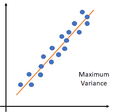
The above figure shows the direction of the maximum variance.
PCA uses the SVD (Singular Value Decomposition) of the data to map it to a lower-dimensional space. SVD decomposes a matrix A (m*n) into three other matrices. Decomposition could also be Eigenvalue based, where a matrix is broken into the set of eigenvector-eigenvalues (Ax = 𝞴x). These are what lead to dimensionality transformation.
The principal components are the perpendicular (orthogonal) axis of the new subspace with fewer dimensions in the directions of maximum variance. These are the new feature axes which are orthogonal to each other, essentially the linear combinations of the original input variables.
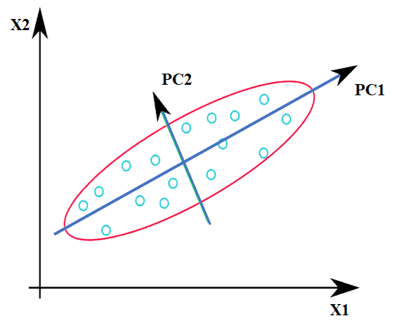
Here, X1 & X2 are the original features, and PC1 & PC2 are the principal components. In simple words, since variance along PC1 is maximum, we can take that as the projected feature (single dimension) instead of having two features X1 & X2.
Python Example
Dimensionality reduction using PCA can be performed using Python’s sklearn library’s function sklearn.decomposition.PCA(). Let’s consider the following data:
| import numpy as np import matplotlib.pyplot as plt # creating the dataset a = np.random.RandomState(2) a1 = a.rand(2, 2) a2 = a.randn(2, 500) x = np.dot(a1,a2).T plt.scatter(x[:,0], x[:,1]) plt.show() |
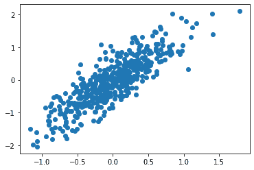
This is a two-dimensional dataset consisting of 500 data points. The relation between these two features of the data is almost-linear. It can be visualized as:
We can use PCA to quantify the relationship between the two features. This is done by finding the principal axes in the data. That can then be used to describe the dataset. Using sklearn, for the above data, it is done as:
| # applying PCA from sklearn.decomposition import PCA pca = PCA(n_components=2).fit(x) |
We can then view the PCA components_, i.e., the principal axes in the feature space, which represent the directions of maximum variance in the dataset. These components are sorted by explained_variance_.
| print(pca.components_) |
Output:
| [[ 0.49794048 0.86721121] [ 0.86721121 -0.49794048]] |
explained_variance_ is the amount of variance explained by those selected components above. This is equal to n_components largest eigenvalues of the covariance matrix of x. To look at the explained_variance_ value:
| print(pca.explained_variance_) |
Output:
| [0.68245724 0.04516293] |
Now, let’s perform dimensionality reduction using PCA. Let’s reduce the dimensions from 2D to 1D. Look at the code below:
| pca = PCA(n_components=1).fit(x) pca_x = pca.transform(x) |
It has been transformed into 1D shape. We can view the components_ and explained_variance_:
| print(pca.components_) print(pca.explained_variance_) |
Output:
| [[0.49794048 0.86721121]] [0.68245724] |
To visualize this dimensionality reduction, an inverse transform of this reduced data can be performed and visualized along with the data points of original x. This is done as:
| x2 = pca.inverse_transform(pca_x) plt.scatter(x[:,0], x[:,1], alpha=0.3) plt.scatter(x2[:,0], x2[:,1]) plt.show() |
Output:
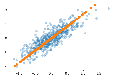
We can see that it is linearly transformed into a single dimension along the principal axis
Summary
In this article, we looked at Dimensionality Reduction using PCA. In the next article, we will focus on Dimensionality Reduction using tSNE.