
Solving Multi-Period Production Scheduling Problem in Python using PuLP
Learn how to use Python PuLP to solve the Multi-Period Production Scheduling Problem using Linear Programming.
Manufacturing companies face the problem of production-inventory planning for a number of future time periods under given constraints. This problem is known as the Multi-Period Production Scheduling problem. In manufacturing companies, production-inventory demand varies across multiple period horizons. The main goal is the level up the production needs for the individual products in this fluctuating demand.
The objective function for such a problem is the minimization of total costs associated with the production and inventory. This planning works with the dynamic method. We can determine the production schedules for each period using Linear programming in a rolling way.
In this tutorial, we are going to cover the following topics:
Initialize Multi-Period Production Scheduling Problem Model
Let’s see the Multi-Period Scheduling Production Problem example from Decision Models Lecture 4 Notes. Here is the link to Notes PDF.
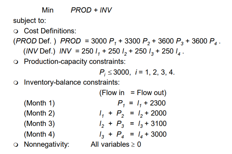
Let’s determine the optimal production schedule by minimizing the total cost using Linear programming.
In this step, we will import all the classes and functions of pulp module and create a Minimization LP problem using LpProblem class.
# Import all classes of PuLP module
from pulp import *

# 1. Initialize Class
model = LpProblem("Minimize Cost",LpMinimize)

# Define production cost, inventory cost, and demand.
quaters = list(range(4))
prod_cost=[3000, 3300, 3600, 3600]
inv_cost=[250, 250, 250, 250]
demand=[2300, 2000, 3100, 3000]
Define Decision Variable
In this step, we will define the decision variables. In our problem, we have two categories of variables quarterly production and inventory. Let’s create them using LpVariable.dicts() class. LpVariable.dicts() will take the following four values:
- First, prefix name of what this variable represents.
- Second is the list of all the variables.
- Third is the lower bound on this variable.
- Fourth variable is the upper bound.
- Fourth is essentially the type of data (discrete or continuous). The options for the fourth parameter are
ContinuousorInteger.
# 2. Define Decision Variables: Production and Inventory
x = LpVariable.dicts('quater_prod_', quaters,lowBound=0, cat='Continuous')
y = LpVariable.dicts('quater_inv_', quaters,lowBound=0, cat='Continuous')
Define Objective Function
In this step, we will define the minimum objective function by adding it to the LpProblem object. lpSum(vector) is used here to define multiple linear expressions. It also used list comprehension to add multiple variables.
# 3. Define Objective
model += lpSum([prod_cost[i]*x[i] for i in quaters]) + lpSum([inv_cost[i]*y[i] for i in quaters])
Define the Constraints
Constraint captures the restriction on the values of the decision variables. The simplest example is a linear constraint, which states that a linear expression on a set of variables takes a value that is either less-than-or-equal, greater-than-or-equal, or equal to another linear expression.
In this step, we will add the production capacity and inventory balance constraints defined in the problem by adding them to the LpProblem object using addConstraints() function.
# Define Constraints
# Production-capacity constraints
for i in quaters:
    model.addConstraint(x[i]<=3000)

# Inventory-balance constraints
model.addConstraint(x[0] - y[0] == demand[0]) # (Month 1)

for i in quaters[1:]:
    model.addConstraint(x[i] - y[i] + y[i-1] == demand[i]) # for (Month 2, 3, 4)
Solve Model
In this step, we will solve the LP problem by calling solve() method. We can print the final value by using the following for loop.
# The problem is solved using PuLP's choice of Solver
model.solve()

# Print the variables optimized value
for v in model.variables():
    print(v.name, "=", v.varValue)

# The optimised objective function value is printed to the screen
print("Value of Objective Function = ", value(model.objective))
Output: quater_inv__0 = 700.0 quater_inv__1 = 1700.0 quater_inv__2 = 0.0 quater_inv__3 = 0.0 quater_prod__0 = 3000.0 quater_prod__1 = 3000.0 quater_prod__2 = 1400.0 quater_prod__3 = 3000.0 Value of Objective Function = 35340000.0
From the above results, we can infer the optimal number of units for each quarter for inventory and production. This is the final solution for the Multi-Period Production Scheduling problem.
Summary
In this article, we have learned about the Multi-Period Production Scheduling problem, Problem Formulation, and implementation using the python pulp library. We have solved the Multi-Period Production Scheduling problem example using a Linear programming problem in Python. Of course, this is just a simple case study, we can add more constraints to it and make it more complicated. In upcoming articles, we will write more on different optimization problems such as network flow problems. You can revise the basics of mathematical concepts in this article and learn about Linear Programming using PuLP in this article. I have written more articles on different optimization problems such as transshipment problems, assignment problems, blending problems.