Basics of Plots.jl and plotting using GPU

Last time we covered Gadfly.jl, which is the library I suggest that you use, due to it’s intuitive approach making it easy to produce interactive and publishable plots. Today we’ll discuss the dominant library for plotting in Julia, Plots.jl.

Introduction

If we were to draw comparisons to the world of Python, then Gadfly is akin to seaborn while Plots is like matplotlib. In fact, Plots is literally a superset of matplotlib. The way plots works are to let you define your visualizations in Julia, and then use a specified back-end to ‘parse’ your visual grammar. This way you can get precisely the combination of features and ease that you wish to deal with. So let’s get started:

Last time we plotted a dataset, this time we’ll instead plot some equations, but lets start of simle:

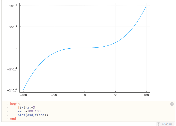
We just defined a cubing function, define an array of 200 elements from -100 to 100, and then pass the two arrays. As simple as that. Creating animated videos is also just as simple. We can iterate through all the pixels in a graph in just 4 lines of code:

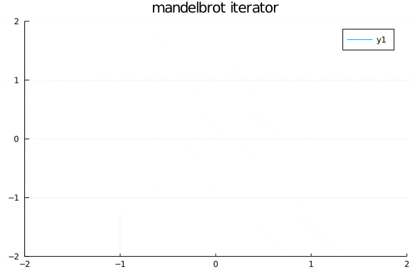
plt=plot(1,xlim = (-2,2),ylim = (-2,2),title="mandelbrot iterator")
@gif for x=-2:1e-1:2,y=-2:1e-1:2
		push!(plt,x,y)
end

But that’s a rather simple example, lets define some functions and plot something more interesting:

Pause here and try to take a guess at what we’re going to do 😉. And lo and behold:

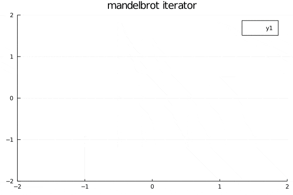
Have you guessed what it is now ? It’s a low-resolution plot of the Mandelbrot set. We generate it using:

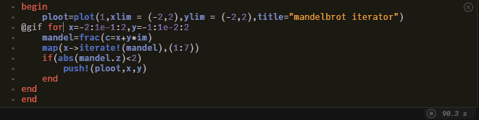
Fun Fact: if you use the non-vectorized version of the above code, your machine will take at least a year to run it. Let’s try to up the resolution just a bit:

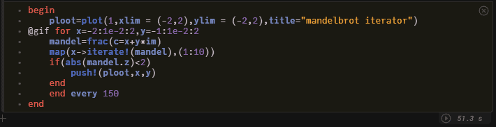
Now, two things. Firstly, did you notice how the higher resolution animation actually takes less time than the lower resolution one? This is common, and hence the best practice is to always draw a joke plot when you begin your session. That way all the libraries are already compiled and good to go when you actually need to plot something. Second, there’s something off about this animation, do you see it? Well, this animation is made up of lines, but our fractal looks more like points. So let’s do that:

All it took was changing plot to scatter:

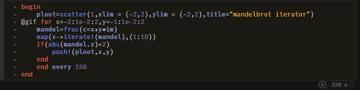
Note how fast all this is, even though we didn’t explicitly use anything GPU based, iterating through 1.2 million complex numbers took less than 5 minutes.

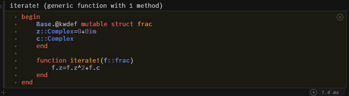
This harks back to the definition of our struct frac if you look carefully, it has only vectorized operations. And this, Julia understands is probably a task for the GPU, and indeed once the heap-size gets too big to fit into the CPU cache, frac is handed over to the GPU, where Plots then deals with it.

You can check that if you change the implementation of frac, julia won’t be able to optimize and you’ll have to wait hours if not years (yes, 1.2 million floating point complex numbers takes about 3.7 years to be handled by my humble 6th gen i5) to generate the above plots.

Now you have a solid foundation of both talking to the data (our last article on Gadfly.jl) and making the data talk via animations.

You can find all this code via the following link

https://github.com/mathmetal/Misc/blob/master/MLG/PlutoPlots