
DBSCAN Clustering
Cluster Analysis comprises of many different methods, of which one is the Density-based Clustering Method. DBSCAN stands for Density-Based Spatial Clustering of Applications with Noise. For a given set of data points, the DBSCAN algorithm clusters together those points that are close to each other based on any distance metric and a minimum number of points.
DBSCAN works on the idea that clusters are dense groups of points. These dense groups of data points are separated by low-density regions. The real-world data contains outliers and noise. It can also have arbitrary shapes (as shown in figures below), due to which the commonly used clustering algorithms (like k-means) fail to perform properly. For such arbitrary shaped clusters or data containing noise, the density-based algorithms such as DBSCAN are more efficient.
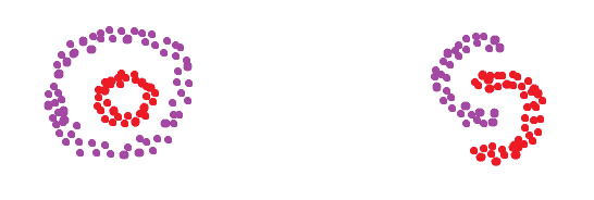
In the above figures, data points are arbitrarily shaped. Density-based clustering algorithms are used to find the high-density regions and group them into clusters
Parameters and Algorithm
DBSCAN Clustering Algorithm requires two parameters:
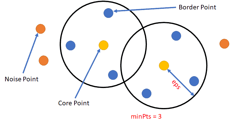
- minPts: The minimum number of data points required for a cluster to form a dense region.
- eps: Distance measure that is used to specify the neighborhood of any data point. If the distance between two data points is less than eps, then those two data points are neighbors.
Hence, after the DBSCAN algorithm, based on these two parameters, there are three types of points:
- Core Points: A data point is said to be a core point if there are at least minPts number of data points within the eps radius.
- Border Points: A data point is said to be a border point that is in the neighborhood of a core point but has fewer than MinPts within the eps radius.
- Noise/Outlier Points: A data point is said to be a noise/outlier point if it is neither a core point nor is in the neighborhood of a core point.
Algorithm:
- Firstly, the parameters minPts and eps are defined
- Arbitrarily pick a starting point from the data, its neighborhood is defined within eps distance and if there are at least minPts number of points within this neighborhood, then this data point is classified as a core point.
- The algorithm continues this for all points. It finds the neighboring data points within eps and identifies the core points. For each core point, if that point is not assigned to a cluster, the algorithm creates a new cluster.
- The algorithm then finds all the neighboring points using the distance metrics; and if there are at least minPts points within eps for the considered data point, then all these points are part of the same cluster.
- The algorithm traverses through the unvisited points. If they are not part of any cluster, then marks them as outlier/noise.
- The algorithm terminates when all the data points are visited.
Example
Let’s take a look at an example of DBSCAN Clustering in Python. The function DBSCAN() is present in Python’s sklearn library. Consider the following data:
| from sklearn.datasets import make_blobs from sklearn.preprocessing import StandardScaler # create the dataset centers = [[2,1], [0,0], [-2,2], [-2,-2]] x, y = make_blobs(n_samples=300, centers=centers, cluster_std=0.4) # normalization of the values x = StandardScaler().fit_transform(x) |
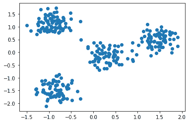
Here, we are creating data with four clusters. The function used to create these data points is the make_blobs() function. The parameters for this function for our data are – 300 sample data points, the standard deviation of a cluster is 0.4, the centers are as defined in the code.
We can visualize these data points using matplotlib, as:
| import matplotlib.pyplot as plt plt.scatter(x[:,0], x[:,1]) plt.show() |
The scatter plot is:
Now, let’s apply the DBSCAN algorithm to the above data points. The python code to do so is:
| from sklearn.cluster import DBSCAN db = DBSCAN(eps=0.3, min_samples=25) db.fit(x) |
Here, for the DBSCAN algorithm, we have specified ‘eps = 0.3’ and ‘minPts = 25’.
Let’s visualize how the points are classified in the clusters:
| y2 = db.fit_predict(x) plt.scatter(x[:,0], x[:,1], c=y2) plt.show() |
The scatter plot is:
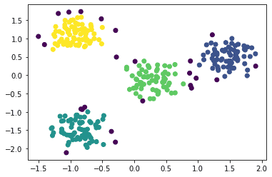
We can see that the algorithm has identified four clusters, marked with Yellow, Green, Dark Blue, and Light Blue colors. The Violet points outside each cluster are the noise/outlier points as detected by the algorithm. By modifying the eps and minPts values, we can get different configurations of the clusters.
Summary
In this article, we focused on DBSCAN Clustering. In the next article, we will look into a Partitioning-based clustering algorithm k-means Clustering.