Transshipment Problem in Python Using PuLP

Learn how to use Python PuLP to solve transshipment problems using Linear Programming.

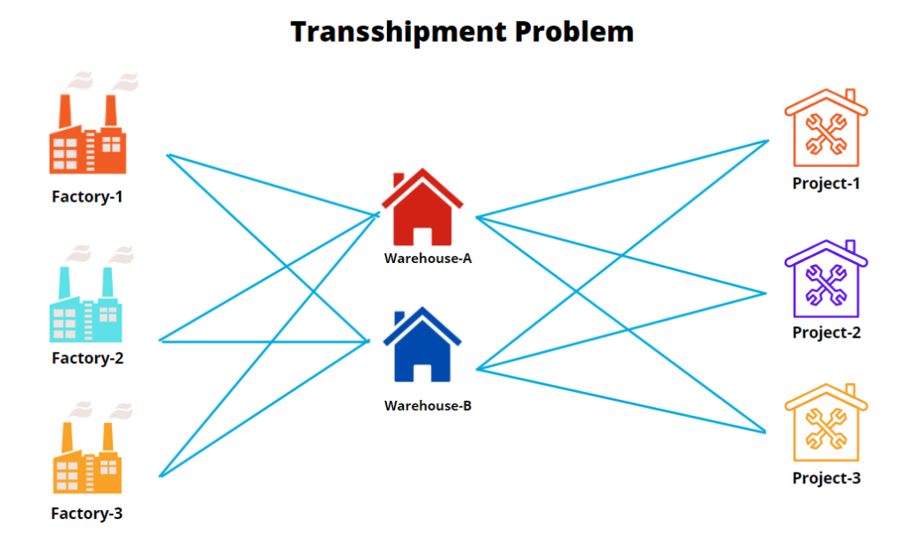
In case of transportation problems, we ship directly the material from source to destination. It means there are no intermediate nodes or points but in real life, we find problems where companies have their warehouses as intermediate nodes. Such problems are known as the Transshipment problems. We can easily turn those problems into transportation problems with some extra constraints and solve the problem.

The transshipment problem is a special case of the transportation problem With intermediate nodes in the shipment paths. For instance, If shipping is happening between New Delhi to Bangalore shipping via Hyderabad may be less expensive than non-stop direct shipping to Bangalore.

In this tutorial, we are going to cover the following topics:

Formulate the Transshipment Problem

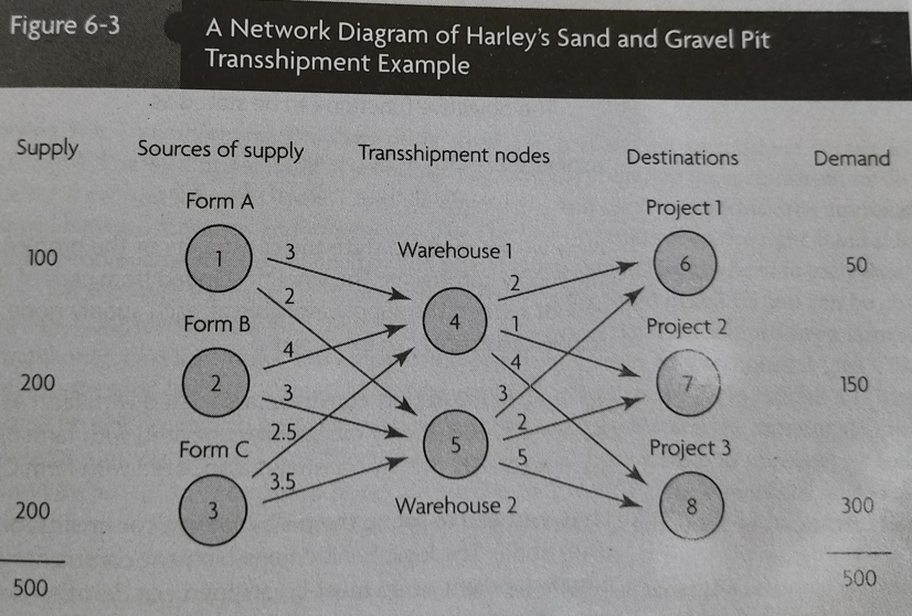
The manager of Harley Sand and Gravel has decided to utilize two intermediate nodes as transshipment points for the temporary storage of topsoil. The following figure shows the network flow diagram (Source):

 # Creates a list of all the supply nodes
factories = ["A", "B", "C"]

# Creates a dictionary for the number of units of supply for each supply node
supply = {"A": 100, "B": 200, "C":200}

# Creates a list of all demand nodes
projects = ["1", "2", "3"]

# Creates a dictionary for the number of units of demand for each demand node
demand = {
    "1": 50,
    "2": 150,
    "3": 300,
}

# Intermediate nodes
warehouses=["P","Q"]

# Creates a list of costs of each transportation path
costs_1 = [  # warehouses
    [3,2],  # A factories
    [4,3],  # B
    [2.5,3.5] # C
]

costs_2 = [  # projects
    [2,1,4],  # P warehouses
    [3,2,5],  # Q
]

# The cost data is made into a dictionary
costs_1 = makeDict([factories, warehouses], costs_1, 0)

# The cost data is made into a dictionary
costs_2 = makeDict([warehouses, projects], costs_2, 0)

Initialize LP Model

In this step, we will import all the classes and functions of pulp module and create a Minimization LP problem using LpProblem class.

# Import PuLP modeler functions
from pulp import *

# Creates the 'prob' variable to contain the problem data
prob = LpProblem("Material Supply Problem", LpMinimize)

Define Decision Variable

In this step, we will define the decision variables. In our problem, we have two lists of variables: Routes from source to intermediate nodes and Routes from intermediate nodes to destination. Let’s create them using LpVariable.dicts() class. LpVariable.dicts() used with Python’s list comprehension. LpVariable.dicts() will take the following four values:

• First, prefix name of what this variable represents.
• Second is the list of all the variables.
• Third is the lower bound on this variable.
• Fourth variable is the upper bound.
• Fourth is essentially the type of data (discrete or continuous). The options for the fourth parameter are LpContinuous or LpInteger.

Let’s first create a list route for the route between warehouse and project site and create the decision variables using LpVariable.dicts() the method.

# Creates a list of tuples containing all the possible routes for transport
Routes = [(w, b) for w in warehouses for b in projects]

# A dictionary called 'Vars' is created to contain the referenced variables(the routes)
vars = LpVariable.dicts("Route", (warehouses, projects), 0, None, LpInteger)

# Creates a list of tuples containing all the possible routes for transport
Routes_2 = [(w, b) for w in warehouses for b in projects]

# A dictionary called 'Vars_2' is created to contain the referenced variables(the routes)
vars_2 = LpVariable.dicts("Route", (warehouses, projects), 0, None, LpInteger)

Define Objective Function

In this step, we will define the minimum objective function by adding it to the LpProblem object. lpSum(vector)is used here to define multiple linear expressions. It also used list comprehension to add multiple variables.

# The objective function is added to 'prob' first
prob += (
    lpSum([vars[w][b] * costs_1[w][b] for (w, b) in Routes]) + lpSum([vars_2[w][b] * costs_2[w][b] for (w, b) in Routes_2]),
    "Sum_of_Transporting_Costs",
)

Define the Constraints

Here, we are adding three types of constraints: supply maximum constraints, demand minimum constraints, and transshipment constraints. We have added the 4 constraints defined in the problem by adding them to the LpProblem object.

# The supply maximum constraints are added to prob for each supply node (factories)
for w in factories:
    prob += (
        lpSum([vars[w][b] for b in warehouses]) <= supply[w],
        "Sum_of_Products_out_of_factories_%s" % w,
    )
    
# The demand minimum constraints are added to prob for each demand node (project)
for b in projects:
    prob += (
        lpSum([vars_2[w][b] for w in warehouses]) >= demand[b],
        "Sum_of_Products_into_projects%s" % b,
    )

# Transshipment constraints: What is shipped into a transshipment node must ne shipped out.
for w in warehouses:
    prob += (
        lpSum([vars[f][w] for f in factories]) - lpSum([vars_2[w][p] for p in projects])== 0,
        "Sum_of_Products_out_of_warehouse_%s" % w,
    )

Solve Model

In this step, we will solve the LP problem by calling solve() method. We can print the final value by using the following for loop.

# The problem is solved using PuLP's choice of Solver
prob.solve()

# Print the variables optimized value
for v in prob.variables():
    print(v.name, "=", v.varValue)
    
# The optimised objective function value is printed to the screen
print("Value of Objective Function = ", value(prob.objective))

Output:
Route_A_P = 100.0
Route_A_Q = 0.0
Route_B_P = 200.0
Route_B_Q = 0.0
Route_C_P = 200.0
Route_C_Q = 0.0
Route_P_1 = 50.0
Route_P_2 = 150.0
Route_P_3 = 300.0
Route_Q_1 = 0.0
Route_Q_2 = 0.0
Route_Q_3 = 0.0
Value of Objective Function =  3050.0

Summary

In this article, we have learned about Transshipment problems, Problem Formulation, and implementation using the python PuLp library. We have solved the transshipment problem using a Linear programming problem in Python. Of course, this is just a simple case study, we can add more constraints to it and make it more complicated. You can also run other case studies on Cargo Loading problems, Staff scheduling problems. In upcoming articles, we will write more on different optimization problems such as assignment problems, balanced diet problems. You can revise the basics of mathematical concepts in this article and learn about Linear Programming in this article.